Blog

  • All the COUNT Functions in Excel

    All the COUNT Functions in Excel

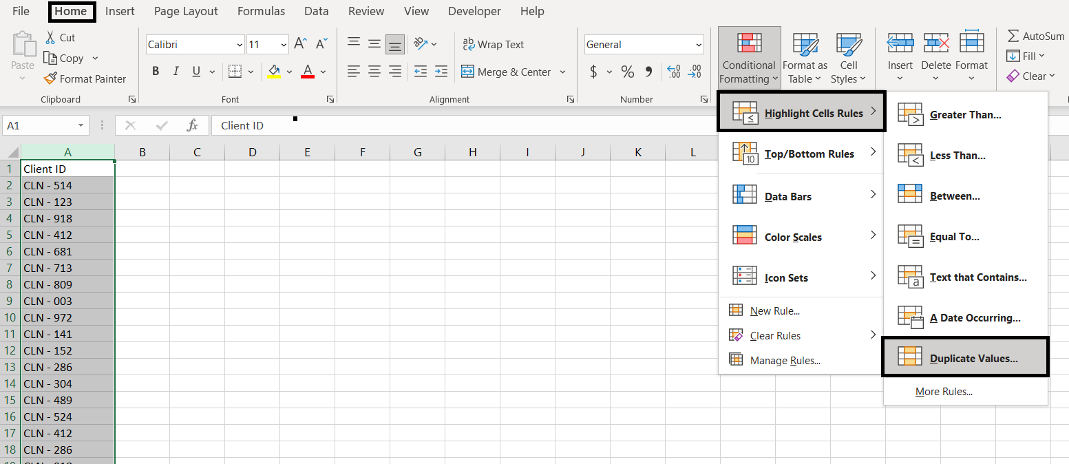
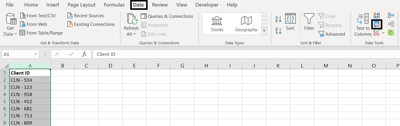
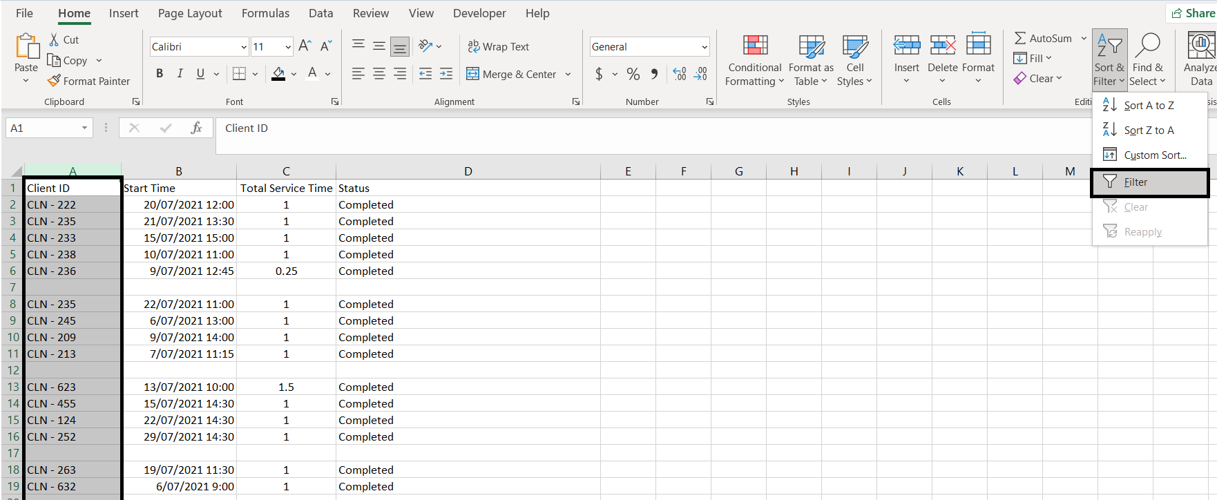
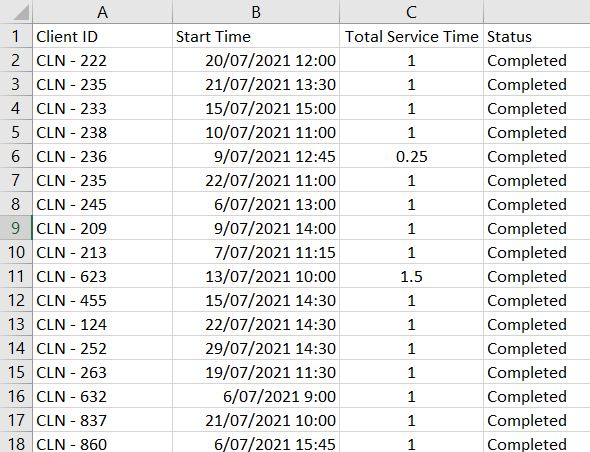
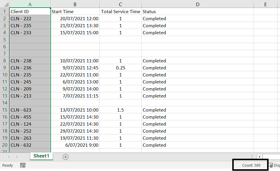
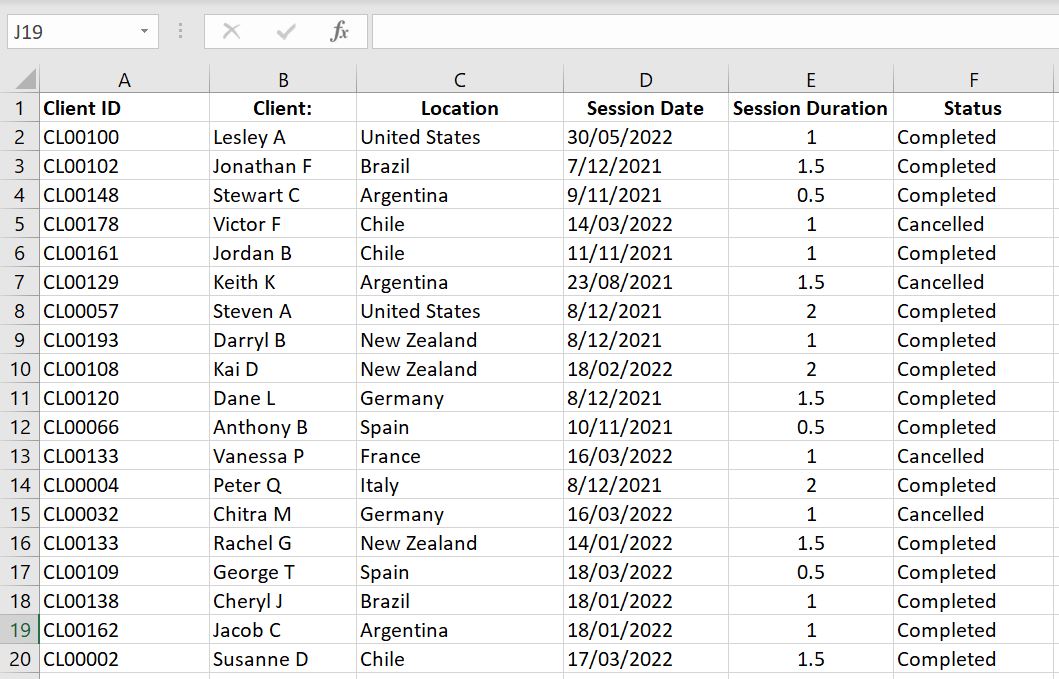
    When it comes to reporting and analysis, the COUNT functions in Excel are a necessity. Very often we need to export reports from a CRM. It could be a report on clients, on open tasks or service activities like below and we need to do analysis and create summary reports with it:

    Excel-Raw-Data-Report

    In this article we will go through the COUNTIF and COUNTIFS, COUNT, COUNTA and COUNTBLANK functions.

    COUNTIF and COUNTIFS

    Do you often export reports from a CRM? And the raw data reports have a full list of entries like the image above. What is the easiest way to calculate how many sessions a particular client attended? How many sessions did a particular client cancelled? How many sessions did a client attend within a specified time period? COUNTIF and COUNTIFS are the perfect functions in Excel.

    • =COUNTIF(range, criteria)
      • This function counts the number of times a particular value appears in a range of cells. In this function, range is the range of cells we want Excel to search in and criteria is the value Excel is looking for in that range
    • =COUNTIFS(criteria_range1, criteria1, [criteria_range2, criteria2], [criteria_range3, criteria3]…)
      • This function is the same as COUNTIF except we can set more than one condition. In this function, we first enter the range of cells we want Excel to search in and then set the value Excel needs to look for. And we can keep going by setting another range of cells and another criteria and so on…
      • Note that criteria_range2, criteria2, criteria_range3 and criteria3 are in square brackets in the function “[ ]” – that is because they are optional. Technically we can set one criteria_range and one criteria, in which case COUNTIFS and COUNTIF are exactly the same.

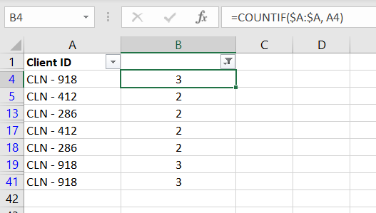
    In the example below, we have =COUNTIF($B:$B, H3) which is to have Excel search through Column B for the value in Cell H3 (“Jonathan F”).
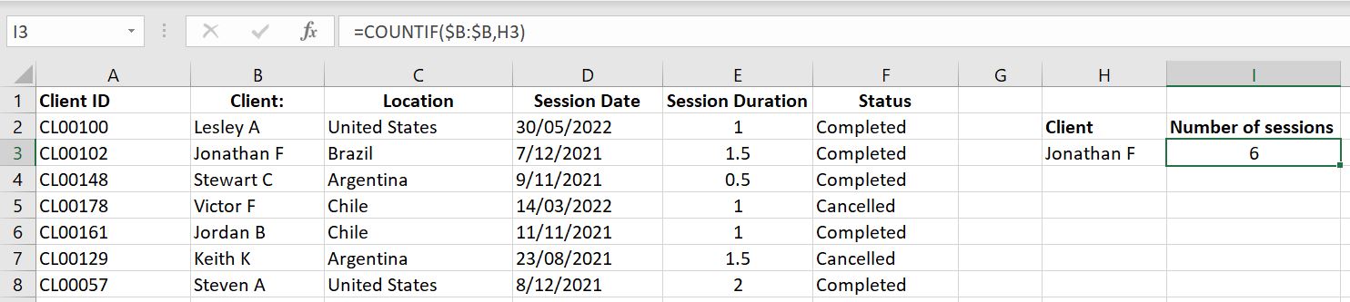
    countif-function-example-Excel

    =COUNTIF($B:$B, H3)

    Using the COUNTIF Function is simple and very useful. But there is one tip to keep in mind:

    Tip: COUNTIF and COUNTIFS functions will only look for exact match. If your COUNTIF/COUNTIFS function returns a 0, make sure the criteria you entered matches exactly with what you have in the range of cells you’re searching. E.g. “Jonathan F” is different to “Jonathan F ” because of the space at the end.

    COUNTIFS is not much different to COUNTIF. Let’s have a look at the example below:

    Excel-countifs-function-example

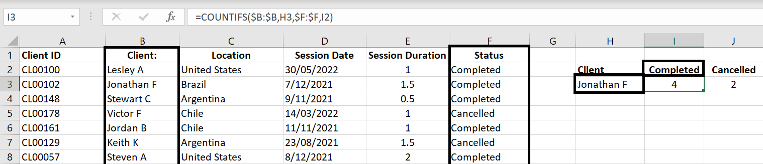
    =COUNTIFS($B:$B, H3, $F:$F, I2)

    Here we entered multiple conditions. We want Excel to search through Column B to find the client’s name and also search through Column F to only count the “Completed” status. And of course we can add even more conditions to it. For example, how many sessions did Jonathan cancel that is of a one-hour duration?

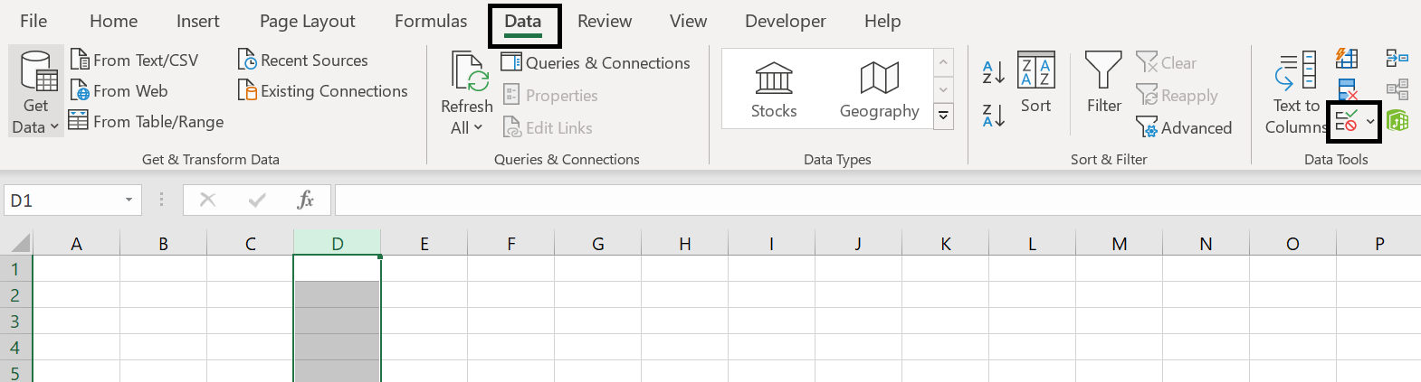
    COUNTIF and COUNTIFS with >, >=, < or <=

    So far we’ve only looked at COUNTIF and COUNTIFS with conditions where the criteria matches exactly with the range of cells specified. But what if we want to count the number of cells where value is greater or less than a certain number? For example what if we want to count the number of sessions that is longer than one hour?

    To demonstrate this, we’ve added clients’ ages in the data and here we want to find out the age demographics of our clients by setting age brackets such as “0 to 18”, “19 to 24”, “25 to 34” and so on:

    countifs-function-greater than-example-Excel

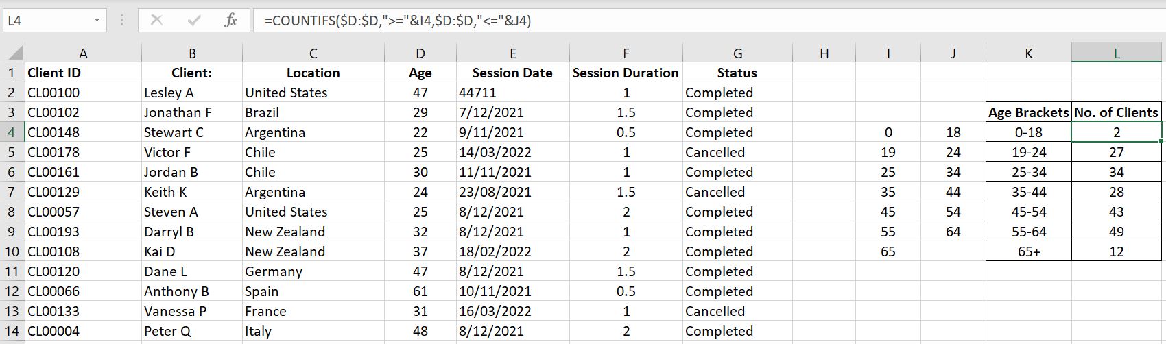
    Let’s break this down. For age bracket 0 to 18, the formula is:

    • =COUNTIFS($D:$D, “>=”&I4, $D:$D, “<=”&J4)

      First condition is to look through Column D ($D:$D) for any value greater or equal to (“>=”&) 0 (Cell I4). And the second condition is to then look through Column D ($D:$D) again but this time for any value less than or equal to (“<=”&) 18 (Cell J4). The result is that we are counting the number of cells in Column D which are between 0 to 18 inclusive.
    Tip: It is always good practice to check our work. The number of clients in Column D should equal to the total number of clients tallied up in the age brackets. If the totals don’t match, consider the following:

    – Are there any blank fields in Column D for any client? If so, do we need to clean up our data? Or do we need an “Unknown” category in our age brackets?

    – Did we miss anything in our formulas such that not all ages are inclusive? E.g. if we put a “>” instead of “>=”, it would mean Excel would be looking for anything greater than but not equal to the value.

    COUNT functions and SUM

    What’s fun with Excel now is that we can now enter an array as the criteria. What that means is Excel will count each criteria in the array for us and list the results one by one. It means you only need to enter the formula once and do not need to autofill or copy the formula down. For example:

    Count-Array-Excel

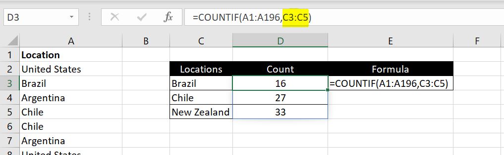
    =COUNTIF(A1:A196, C3:C5)

    Notice in the example above, we entered “C3:C5” as the criteria. And what that does is Excel would calculate the COUNTIF function for C3, C4 and C5 and list the results down automatically in D3:D5.

    And to make things even simpler, instead of doing the COUNTIF function multiple times and then calculating the total at the end, we can now wrap a SUM function around a COUNTIF function. This will help if you don’t care what the COUNTIF result is for each criteria and only want to know the total:

    COUNT-SUM-Excel

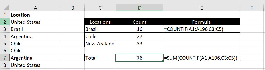
    =SUM(COUNTIF(A1:A196, C3:C5)

    In the example above, we did not need to calculate the COUNTIF function individually for “Brazil”, “Chile” and “New Zealand”. In D7, we can calculate it in one formula by wrapping the SUM function around the COUNTIF function.

    COUNTBLANK

    COUNTBLANK as the name suggests counts the number of empty cells in a range specified. This is useful in checking the data to see if there are any blanks. And will give us a chance to fix these data gaps in our CRM.

    Excel-countblank-example

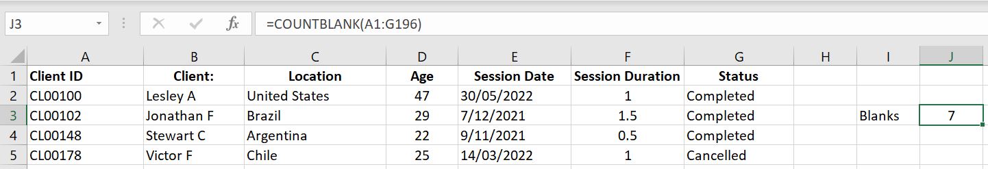
    The function is incredibly simple to use:

    • =COUNTBLANK(the range of cells you want to check if they are empty)

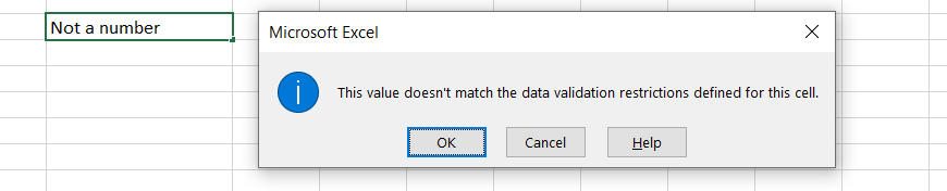
    Once again we will just need to be careful. A cell with a space in it ” ” is not blank according to Excel.

    COUNTA and COUNT

    • COUNTA: counts the number of cells in the specified range that are not blank
    • COUNT: counts the number of cells that contain numbers (0 is a number. Negative numbers are also numbers. Decimals are also numbers)

    Consider this set of random data in range A1:A8:
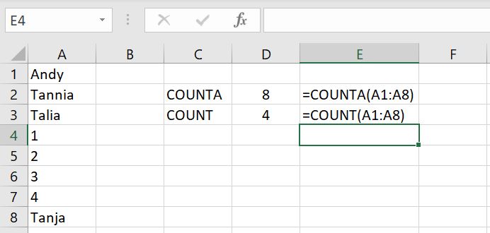
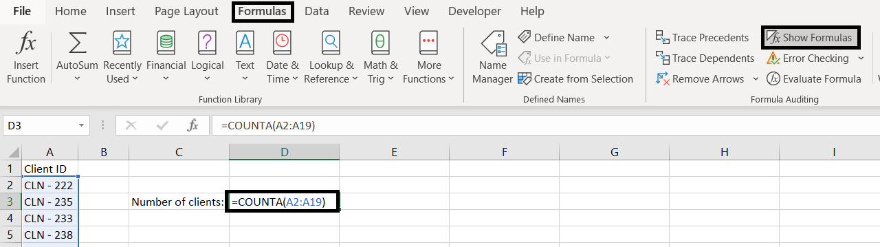
    counta-count-excel-functions-examples

    =COUNTA(A1:A8)

    =COUNT(A1:A8)

    COUNTA returns 8 because all 8 cells have data in them. COUNT returns 4 because only 4 of them are numbers.

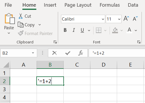
    This little example below show that COUNTA function will also count any cells as not empty if it has formulas in them. In this case, “” is technically equivalent to a blank but COUNTA will still count it as containing data.

    counta-excel-functions-example

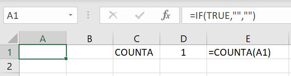
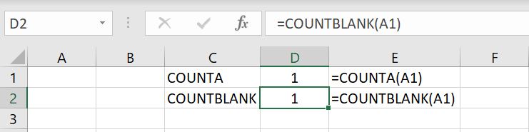
    You would think that using COUNTA and COUNTBLANK, you would always get the total number of entries. But the example above shows that it doesn’t. COUNTA will count A1 above as 1 (because it has a formula in it although the formula returns a “” result) and COUNTBLANK will also count A1 as 1:

    counta-countblank-examples-Excel

    Cell A1: =IF(TRUE, “”, “”)

    With one cell (A1), both functions are returning 1 as a result. Adding them up, you would get a total of 2 although there’s only one cell. So we just need to keep in mind this is how COUNTA function works. As long as there is some value or formula entered into the cell, COUNTA will count it as a non-empty cell. It makes sense. The irony here is that the formula we put in is returning an empty cell.

    We hope you now understand how and when to use each COUNT functions. If there’s more you would like to know about or if there’s more you feel we should add on this topic, please leave a comment below!

  • Easiest Way to Understand VLOOKUP in Excel

    Easiest Way to Understand VLOOKUP in Excel

    What is VLOOKUP in Excel? How do you use it? And when should you use it? In this article, we will go through all that. And in the end we will also go through common errors you could get with the VLOOKUP function.

    What is VLOOKUP in Excel? (And its limitation)

    VLOOKUP is a built-in function in Excel. This function looks for a value of your choice in a column from top to bottom and once that value is found, it returns any value to the right in that row. In other words, Excel starts in the leftmost column, top to bottom Excel looks for the lookup value and then once the value is found, it moves to the right:

    what-is-vlookup-excel

    The limitation with VLOOKUP is that once the value of your choice is found in a column, it can only return a value on the right-hand side of that cell. Using the example above, given the name of a staff, we can find the staff’s Start Date and Employee Number. But we will not be able to use the Employee Number or Start Date to find the staff’s name.

    How Does VLOOKUP Work?

    Let’s jump straight into it. The VLOOKUP function is:

    • VLOOKUP = (lookup_value, table_array, col_index_num, [range_lookup])

    The easiest way to understand this is:

    • Excel will look through the first column in our table of data (table_array) to find a value of our choice (lookup_value). Once found, it will move to the right to return the value in x column (col_index_num). [range_lookup] is an option we have whether we want Excel to find an exact match (FALSE) or an approximate match (TRUE) with our lookup_value. If left blank, by default it will be true.
    Tip: to use approximate match with VLOOKUP (TRUE), your table must first be sorted alphabetically or numerically.
    Tip: when looking through the first column in the table_array, VLOOKUP will start from top and will stop once the lookup_value is found. That means if we have multiple rows with that same lookup_value, VLOOKUP function will stop at the first one it finds starting from the top.

    Let’s put this in practice:

    Excel-Vlookup-Example

    With the example above: VLOOKUP(E2, $A2:$C, 3, FALSE):

    • Excel is looking for value in E2 (“Kate N”) in the Column A (first column in table A:C). Once it finds “Kate N” which in this case is in row 10, it returns the value in the 3rd column (as we have specified). Column A is 1st column, B is 2nd column and C is 3rd column.

      Note: hypothetically if the table_array is F1:L100, F would become 1st column, G becomes 2nd column, H becomes 3rd column, I becomes 4th…and so on.

    If we have a range of lookup values listed down as a column or across as a row, we could enter that range as the lookup_value. In the example below, we’ve selected E2:E5 as the lookup_value and Excel automatically each lookup_value for us one by one:

    Vlookup-multiple-lookups-excel

    But alternatively we could of course always put E2 as the lookup_value and drag the formula down. In that case, just remember to lock in the table_array with absolute referencing. Otherwise the table_array would shift:

    Excel-Vlookup-Shift-Table_array

    Because we entered A1:C50 as the table_array in the first VLOOKUP function in F2, as I dragged the formula down to F5, the table has then shifted down one row by one row to eventually become A4:C53. But because “Susan W” is in row 3, it is no longer part of that table_array. To fix that, simply add $ signs to the table_array so it’s fixed:

    Excel-Vlookup-absolute-referenced-Table_array

    As you can see, the VLOOKUP function is not too hard to use. Now let’s have a look at the common errors you could get with VLOOKUP

    Common Errors with VLOOKUP

    #NA – Cannot Find The Value

    #NA is probably the most common error you would find with VLOOKUP. It simply means the lookup_value cannot be found. Here’s a few reasons why:

    The lookup_value cannot be found. With the example below, there’s no “Kate” in Column A:

    Excel-Vlookup-error-cannot-find-lookup_value

    The example below is not as obvious and is probably one that confuses most people because “Kate N” is clearly in Column A (row 10). The issue is that with exact match, Excel really needs the lookup_value to match the value in column A exactly. In E2, the lookup_value is actually “Kate N ” and the value in column A is “Kate N”. The space at the end, “Kate N ” means it is not the same as “Kate N”.

    Note: Excel will also return #NA if we have two spaces in between “Kate” and “N” such as “Kate N”.

    Excel-Vlookup-error-cannot-find-lookup_value-trim

    In these cases, check your lookup_value to make sure it matches exactly with what is in Column A. Useful tip: you could add a dropdown list of column A in the lookup_value cell. This way you are guaranteed that the value will match. If you want to know how to add a dropdown list, check out Dropdown List in Excel.

    Besides from the lookup_value, also make sure your table_array is correct. Remember Excel will only search for the lookup_value in the leftmost column in the table_array. In the example below, the table_array is A1:D100 and column A does not have “Kate N”.

    Vlookup-error-wrong-table_array-Excel

    In the example below as well, column B also does not have “Kate N”:

    Excel-Vlookup-error-wrong-table_array

    #REF – Referenced Cell is not Valid

    It’s not as often that you get a #REF with VLOOKUP. With all #REF, it is because an invalid cell is referenced. This happens when col_index_num is outside the table_array.

    As an example below, the table_array is A1:C100 which means Column A is col_index_num 1, Column B is col_index_num 2 and Column C is col_index_num 3. Because we only have columns A to C, when we enter 4 (or beyond) for col_index_num, a #REF is returned.

    Excel-Vlookup-ref-error-invalid-cell-referenced

    #VALUE – Unexpected Input in the VLOOKUP Function

    Hopefully you will never see this. Unlike with #REF above where we put down a col_index_num beyond the table_array, this time we have gone the other way around. The first column in the table_array is col_index_num 1, the second column is col_index_num 2, third is col_index_num 3…and so on. The idea is it starts with 1 and can go to however big your table_array is. But it can never be less than 1. If you enter 0 or a negative number for col_index_num, you will get a #VALUE.

    Excel-Vlookup-value-error

    We hope you now understand how the VLOOKUP function works and more importantly know when to use it and how to avoid getting an error. For any feedback on this article, please leave a comment below!

  • How To Set Up A Searchable Dropdown List?

    How To Set Up A Searchable Dropdown List?

    In the Dropdown List in Excel article, we went through the basics of setting up a dropdown list in Excel. This time we will go through how to make a searchable dropdown list and we will also sort the list in alphabetical order so it is easier to search through the list. And then at the end we will set up an even more complex dropdown list where the list of options changes depending on another cell and is searchable.

    Creating a Searchable List

    long-list-of-entries-excel

    As an example above, let’s say there’s a very long list of entries in column A. Creating a searchable list will make it a lot easier to look through the column. To do this, we first use the SEARCH function to look for that keyword/key phrase in the list. And then we use the ISNUMBER function to see if each item in the list returns a TRUE response or a FALSE response. TRUE means it can be found. FALSE means it cannot be found. Then we use the FILTER function so that we only see the TRUE response list. And then at the end we use the SORT function to sort the end result in alphabetical order.

    To make it easier to understand, have a look at example below:

    Search-List-Full-List-Dropdown-Excel

    The formula:

    • =SORT(FILTER(A2:A34,ISNUMBER(SEARCH(F2,A2:A34)),”Not found”))

    The formula looks for what is entered in F2 (Keyword) in the A2:A34 list. If anything can be found, the A2:A34 list will be filtered to return the new list. Tip: if there is no keyword or key phrase entered at all, the full list will appear. And if nothing can be found, the list will return with “Not found”.

    Search-List-Dropdown-Excel

    Search-List-Dropdown-Not-Found-Excel

    Put this New Searchable List into a Dropdown List

    To make this searchable list a dropdown list, it is simple. Select the cell where you want to create the dropdown list, go to Data at the top and select Data Validation:

    Dropdown-list-data-validation

    Tip: Because we don’t know how many items will be returned based on the keyword or key phrase, the list is dynamic. We know the list starts with C2 and then we can add # after it. This way Excel will include everything from C2 to the last item in the list, whatever that is.

    In the Error Alert tab, make sure the “Show error alert after invalid data is entered” is not ticked.

    Dropdown-list-error-alert-data-validation

    Now we have a dropdown list which is searchable.

    Searched-Dropdown-List-Excel

    Searched-Dropdown-List-Not-Found-Excel

    Creating a Dynamic Searchable Dropdown List

    Combining everything we’ve learned, we will now make a dropdown list where the list of entries changes depending on value of another cell and is searchable. Continuing on with the example above, in the real world a staff directory is usually separated by teams. So how can we have a dropdown list where the list of staff is different depending on which team is selected? And of course we want the list to be searchable.

    For example: the first dropdown list allows you to select one of the teams that is available across Row 1 (A1:E1):

    First-Dropdown-List-Excel

    And the second list “Staff” changes depending on which team you’ve selected in J2:

    Second-Dropdown-List-Excel

    To do this, we really only need to add one more step to above. Because there are now multiple lists available, we now need to create this one list which updates itself depending on which team is selected:

    Search-List-Depending-On-First-Dropdown-Excel

    The formula is:

    • =INDEX($A$2:$E$8,ROW($A$1:$E$8),MATCH($J$2,$A$1:$E$1,0))

    This…looks ugly. The #REF does not matter because when making this list searchable, the #REF will return a FALSE result hence it won’t show up in the final dropdown list. But the 0 will if no keyword/key phrase is added – because the full list appears when nothing is entered. To fix this, we just need to add an IF formula. IF a 0 is returned, give us blank “” instead.

    • =IF(INDEX($A$2:$E$8,ROW($A$1:$E$8),MATCH($J$2,$A$1:$E$1,0))=0,””,INDEX($A$2:$E$8,ROW($A$1:$E$8),MATCH($J$2,$A$1:$E$1,0)))

    Updated-List-Depending-On-First-Dropdown-List-Excel-index-match-no-zeroes

    As mentioned, it doesn’t matter if the #REF is there. But if you like to see a cleaner list, you can use the IFERROR formula so that any error will also return “” – blank.

    The next step is to make this new list searchable. Here we follow the exact same steps as what we’ve shown in the beginning of this article. First we search for what is entered in K2 in the new G2:G8 list. Then we see if a TRUE or FALSE response is returned. And then we filter to have a list with the TRUE responses. At the end we sort the list alphabetically.

    Search-Dynamic-List-Dropdown-Excel

    Again, we need to go into the Error Alert tab and make sure the “Show error alert after invalid data is entered” box is not selected.

    Search-New-Dynamic-List-Dropdown-Data-Validation-Excel-2

    To make the file look cleaner, you can hide column G and H. Sometimes we set this up in a separate worksheet tab and protect the sheet so no one would accidentally change or delete the formulas. For information on how to protect a worksheet, you can check out How to Password Protect an Excel File.

    Excel-Searchable-Dynamic-Dropdown-List

    We hope we have made it clear on how to make a searchable dropdown list and how to have the list changed depending on the value of another cell. If anything is not clear, feel free to leave a comment below!

  • How to Password Protect an Excel File

    How to Password Protect an Excel File

    This is a step by step guide on how to password protect an Excel file. Apart from setting password for the whole workbook, we will also walk through how to restrict access (with or without password) for specific worksheets and even specific cells. First it is important to distinguish the difference. With setting a password on the entire workbook, no one will be able to open the file again unless a password is entered. No one will even be able to see the content. With Protect Sheet, content can still be viewed but user will not be able to make any changes to the data unless the worksheet is unprotected again.

    Password Protect the Entire Excel File

    It sounds obvious but remember that when we add a password to the entire Excel file, the next time we open the file we will be asked to enter the password before being able to see any content in the workbook. Make sure you remember this password or you have it saved somewhere. To add a password to the entire file:

    1. Click on File
    2. Select on Info
    3. Select Protect Workbook > Encrypt with Password:

      password-protect-excel
    4. We will then be asked to enter the same password twice

    The next time we want to open the file, we will be prompted to enter password before we can open the file:

    password-protected-file

    How to Deactivate Encryption

    We cannot deactivate the encryption until we open the file. This of course means we must enter the password first. Once the file is open:

    1. Go to File
    2. Click on Info
    3. Select Protect Workbook > Encrypt with Password:

      Deactivating-Password-Encryption-Excel
    4. Clear the existing password in the field
    5. Click Ok.
    Note: And because this means anyone can remove a password once the workbook is open, if the Excel file is highly confidential, we recommend you to check the encryption every time you close a file to make sure it is still password protected.

    Protect Sheet in Excel

    Protecting worksheet is another built-in feature in Excel. We can prevent people from making any changes to the entire worksheet or to specific cells in a worksheet. Others are essentially given read-only access. This may not necessarily be for security reasons but simply because there are many data and formulas in the worksheet we don’t want others to accidentally make changes to. For this reason you should consider whether it is necessary to add a password. After all adding a password only means we will now have another password we need to remember.

    To protect our sheet:

    1. Go to the Review tab
    2. Click on Protect Sheet:

      review-tab-excel
    3. We can now enter a password if we wish. However we can also leave it blank. Underneath the password, we can choose what we still want to allow users to do after worksheet is protected. By default the following will be selected. This means users will still be allowed to select cells (hence can copy content) even after worksheet is protected.

      protect-sheet-excel
    4. Click OK

    With the above settings, we can select cells in the worksheet. But if we double-click or try to enter any content, we will receive the follow message:

    password-protect-message-excel

    How to Unlock Specific Cells

    We also have the option to only lock certain cells in a worksheet. This is particularly useful when we have formulas in the worksheet but we also require users to enter data.

    Before protecting the sheet:

    1. Select the cells we want to allow users to edit
    2. Right-Click and select Format-Cells. Alternatively press Ctrl + 1
    3. In the Protection tab, deselect the Locked tickbox:


    4. Click OK
    5. Protect Sheet by clicking on Review tab at the top > Protect Sheet > Click OK

    In the example below, we’ve “unlocked” the highlighted columns and hence we can enter data. However when we try to enter data into any other cell, we will receive an error message:

    unlock-protected-cells-excel

    As we can see with the image above, almost everything at the top is greyed out. Even with the unlocked cells, we can only enter data. We cannot do any formatting (e.g. changing font, merging cells or insert rows/columns). Here’s something we can do to change that and it really all depends on how much access we want users to have:

    When we click on Protect Sheet, we can have the following selected and deselected:

    select-unlocked-cells-excel

    As we can see above, with these settings we are allowing users to select unlocked cells and format cells. And image below shows the results – users will have the option to format unlocked cells. Note that because the “Format cells” box is ticked, users can technically format any cells in the worksheet. However because the “Select locked cells” is not ticked, users cannot even select the locked cells hence they are not able to format/edit locked cells. Please also keep in mind because users cannot select locked cells, they will not be any to copy any content. As you can imagine, there are different variations available for us depending on our specific needs.

    formatting-unlocked-cells-excel

    How to Unprotect Sheet

    Unprotecting Sheet is simple:

    1. Go to Review tab
    2. Select Unprotect Sheet – if a password was added when worksheet was protected, we will need to enter password to unprotect the sheet.

    Protect Workbook – Ability to Insert/Delete/Hide/Unhide Worksheets

    Aside from encrypting the entire Excel file and protecting a particular worksheet, we can also “protect workbook”. And this means not allowing users to insert, delete, rename, hide, move/copy or unhide worksheets. Similar to protecting sheet, we have the option to add a password or to protect without a password.

    1. Go to Review tab
    2. Select Protect Workbook
    3. Click OK – with protecting workbook, we do not have many options on the settings. We can choose to enter a password but it is optional

    Once workbook structure is protected, usual functions we can do with a worksheet will be greyed out:

    protect-workbook-excel

  • How To Identify Duplicates in Excel

    How To Identify Duplicates in Excel

    What is a simple way to identify duplicates in Excel? In this article, we will go through two ways of doing that: using Conditional Formatting and COUNTIF function. And at the end we will look at how we can find the total number of unique values in a list.

    Finding Duplicates with Conditional Formatting

    The easiest way to finding duplicates in a column is to use conditional formatting:

    1. Highlight the column
    2. Go to Conditional Formatting > Highlight Cells Rules > Duplicate Values

      identify-duplicates-conditional-formatting
    3. Select the formatting we want for cells that contain duplicates
    4. Click OK

    After conditional formatting is applied, we can add Filter to the column and filter by cell color:

    filter-by-color-excel

    And then we can do the cleaning up we need. We can start from the top and delete each duplicate row. But before doing so, we suggest sorting the data in order first. You can do that by going to the Home tab > Editing section > Sort & Filter > Sort A to Z:

    Sort-Column-Excel

    Why do we need to do this? We want to sort the list in order first so then we can group each set of duplicates together. This is not a mandatory step but it does make it very clear how many duplicates there are for each item and hence gives us an indication on how many duplicated row we will need to remove for each.

    Note: when deleting duplicates, do not delete more than one row at a time because we only want to delete the duplicated cell. The idea is when we delete/clear one cell, because there will be no more duplicate (assuming there is only one duplicate), the conditional formatting for the second cell will disappear.

    Finding Duplicates using COUNTIF function

    Conditional formatting certainly helps with identifying the duplicates but it does not tell us how many duplicates there are for each cell. This is something the COUNTIF function can do:

    countif-duplicates-excel

    =COUNTIF($A:$A, A2)

    Because we are counting that item which is inside the list itself, the COUNTIF function will not return a number lower than 1. So if we want to precisely calculate how many duplicates there are for a particular value, we can add a “- 1” at the end of the formula. For example above: “=COUNTIF($A:$A, A2) – 1”. Afterwards we could apply Filter and filter out values that have no duplicates:

    duplicates-countif-filter-excel

    Counting Unique Values

    Above is the most common method we use to identify duplicates. To then count the number of unique values, we usually do one of the following:

    Copy the column and paste it on another sheet. Having the column highlighted, go to Data tab > select Remove Duplicates:

    remove-duplicate-excel


    And Excel will tell us how many unique values there are in the list. We can see below Excel has very cleverly excluded the heading of the column so we know the 36 does not include the heading.


    unique-number-remove-duplicates-excel

    Have we missed anything on this topic? If you find that we have missed anything, or if you have any questions, want us to include anything else into this article or need clarification on anything here, please let a comment below! We want to keep improving our content so it is useful for everyone.

  • Why Is Excel Showing the Formula Instead of the Result?

    Why Is Excel Showing the Formula Instead of the Result?

    There could be a few reasons why Excel is showing the formula instead of the result. First of all, all formulas in Excel must start with the equal sign “=”. Make sure there is nothing before the equal sign. Especially if there is an apostrophe ( ‘ ) in front, in Excel (and also in other programming languages), apostrophe turns a formula or a line of code into a comment or text so the program will not run the formula or code.

    Cell is in TEXT format

    This is the most common reason why Excel is showing formulas instead of the results. It happens most often when a report is exported from another system, perhaps in a CSV format. When entering a formula, it will by default be in a TEXT format:

    text-format-excel-showing-formula

    To resolve this, change the format to General and enter the formula again:

    Show Formulas is Enabled

    This is a less common explanation (but maybe someone is playing a prank on us, who knows?) If we go to the Formulas tab, we need to make sure Show Formulas is not selected:

    show-formula-selected

    Simply deselect the Show Formulas button and we shall see the end result of the formula instead of the formula itself.

    The Apostrophe – All Formulas Must Start With An Equal Sign

    Excel will only recognize a function or a formula and calculate it if it starts with an equal sign. That means if in a cell, we type in “1+2”, Excel will not do the calculation for us. It will simply remain as “1+2”. To have Excel do a calculation, it must start with an equal sign. Using the same example, we must enter “=1+2”.

    But what if we want to enter a formula or a function into a cell and do not want Excel to calculate it? Well here we can add an apostrophe in the beginning. And the apostrophe won’t appear in the cell. What the apostrophe does is that it tells Excel this is a text and not a formula to be calculated:

    Excel-apostrophe-text

    Have you ever entered a value in Excel that starts with 0? For example: “007” and then Excel just removes the 0s for us and leaves the cell with 7. That is because Excel automatically recognizes “007” as a number. There are two ways we can change this and keep the 0s in front:

    1. Change format of the cell into Text:

      Text-Format-Excel

      With that, whatever we enter into the text, it will appear exactly the way we put it
    2. Another way, a quicker way, would be to simply put an apostrophe before typing in the value. For example: ‘007. This will also have Excel recognize that this cell is now in a text format.

    We hope this has helped you in understanding why formulas are not calculating and why Excel is showing the formulas and not calculating it. If you have gone through this article and none of these situations are applicable, feel free to leave us a comment below! We want to keep improving our content and make it more complete. So if there are other common scenarios where Excel is showing the formula instead of calculating it, please share with us!

  • How To Remove Empty Rows in Excel

    How To Remove Empty Rows in Excel

    What is the best way to remove empty rows in Excel? There is a couple of different ways to do it. One way involves using Visual Basic Applications (VBA) and the other way doesn’t. In this article, we will go through both methods on how to remove empty rows.

    Removing Empty Rows

    The first method we will go through does not require VBA. It means this method is most likely easier to follow as no coding is required. However if removing empty rows is repetitive task that you need to do time and time again, you might want to consider creating a VBA for it. With VBA, it means the whole process can be simplified into a click of a button.

    To remove empty rows:

    1. Apply filter to the whole table by first highlighting the whole column and click Filter. Alternatively use hotkey (CTRL & L) to apply Filter:

      applying-filter-excel

      Note: it is important highlight the entire column first. Because the table is currently separated by empty rows, if we do not select the entire column, Excel will think the table ends at the first empty row. Example:

      wrong-filter-excel

    2. Filter to (Blanks):

      filter-blanks-excel
    3. Highlight all empty rows. You can do this by first:
      • Select the first empty row:

        Highlight-Row-Excel
      • Hold the SHIFT key
      • Select the last empty row
        Highlight-All-Empty-Rows-Excel
    4. Right-click and click on Delete Row:

      delete-empty-rows-excel
    5. Remove Filter:

      remove-filter-excel

    Here we can see that all the empty rows in the table are now removed.

    Remove Empty Rows Using VBA

    To use VBA, we will first need to make sure Macro/VBA is enabled. Once Macro/VBA is enabled:

    1. Go to Developer tab and open Visual Basic
    2. Insert a new module
    3. Copy and paste following into the module:

    Sub remove_empty_rows()

    Dim i As Integer

    For i = 1 To 600 ‘change 600 to the last row of the table. See below (A)

    If Len (Cells(i, 1)) = 0 Then ‘Cells(row, column). In our example, the empty cell is in Column A hence it is Cells(i, 1). If it is Column B, it would be Cells(i, 2). And so on…

    Rows(i).Delete

    If i = 590 Then ‘change 590 to the total number of items in Column A and + 1. See below (B)

    Exit For

    Else

    i = i – 1

    End If

    End If

    Next i

    End Sub

    A) In this For loop, “For i = 1 to 600” is telling Excel to loop from number 1 to 600 and because we are putting i in Cells(i, 1), we are looping from row 1 to 600. And of course this can change depending on which row our table starts and ends.

    In this example the last row of the table is 600 hence we are looping from 1 to 600

    B) This number needs to be the total number of items in the column + 1. To find out, highlight the relevant column, check the “Count” at the bottom and + 1.

    row-count-excel

    In this case, there are 589 items in the column hence we need 590 (589 + 1). Explanation: And this is the row number we need to tell Excel to stop and exit the For loop. This section is here to account for situations where we may have multiple consecutive blank rows. Hence every time a blank row is deleted, instead of moving onto the next row number (next i), we want to check the same row again to see if it is also blank (hence we need i = i – 1). However this can create an endless loop where “i” will never get to 600 if we keep looping i = i – 1. But if we already know that there are only 589 items in the whole column then we can confidently tell Excel to exit the For loop at row 590.

  • Using Data Validation in Excel

    Using Data Validation in Excel

    Data validation in Excel allows us to set parameters on what can be entered into a cell and we can also choose what happens when invalid data is entered. This is very useful in keeping the data tidy. We have more predictable data which can help with future analysis and calculation. As a quick example, if we want to collect data on how many pets each person has, we may end up having data such as “one”, “2”, “2 dogs”, “none”. With data validation, we can make sure only whole numbers can be entered.

    How To Set Validation Criteria On Cell(s)

    To set up data validation:

    1. Highlight the cells (or range of cells) we want to apply data validation on
    2. Go to Data tab and select Data Validation:

      data_validation_setup
    3. By default of course, data validation would allow “any value” to be entered. Here in the “Allow” field, we can change that. Have a look at the list below

      data_validation
    Whole number & Decimal

    With whole number & decimal, we can make sure only numbers are entered into the cell. Of course choose wisely whether whole number or decimal should be selected. With example given at the very top, if we want to count the number of pets each person does, having decimals would not make much sense so whole number would be preferred.

    Once whole number or decimal is selected, we will need to set further parameters around what numbers can be entered.

    data_validation_numbers

    Again this can be particularly useful as we can further narrow down what can be entered. As an example if we are collecting data on how many days people are exercising in a month, it will be wise to set the parameter between 0 to 31 as you can’t have negative days or more than 31 days in a month.

    If we want to allow a wide range of numbers to be entered, we can always set whole number/decimal between -100000000000 to 100000000000.

    Date & Time

    Date and time are similar to whole number and decimal. Once we selected either one, we will need to set further parameters to narrow down what can be entered. For example we can set validation criteria so that only time can be entered and must be greater than 6pm

    Tip:

    In Excel, 1 is represented as 1 day (24 hours). So 6pm (18:00) as a number is 3/4 (18/24) as a number. For more information, you can read more here: Date/Time in Excel. What it means here is if we set “greater than” 18:00 as validation criteria, Excel will allow us to enter any value greater than 0.75 even including 421 or 129 or 492 although these numbers are clearly not a time.

    To solve this, instead of using “greater than”, use “between” and set end time as 23:59. Doing this you will be able to prevent users from entering numbers such as 1 or greater. Fractions can still be entered as long as when converted back into time, they fall within the validation criteria.
    List

    This allows us to add a dropdown list. You can find more information here: Dropdown List in Excel. On that page, we go through how to add a dropdown list using data validation. And also how to add a dropdown list where the list changes depending on the value in another cell. For example:

    data-validation-two-dropdown-lists

    What To Do When Invalid Data Is Entered

    We can also choose what happens when invalid data is entered. Go to the Error Alert tab after clicking on Data Validation:

    data-validation-error-alerts

    By default, Excel will always stop invalid data from being entered. An error message will pop up and the invalid data will be removed from the cell. In the Title and Error message fields, we can customize the message

    Warning and Information are rather similar. Once invalid data is entered, an error message will still pop up. However we would have the option to allow or remove the data.

    data-validation-information-alert

    If we click “OK”, we are acknowledging the invalid data and allowing it to be entered. But if we click Cancel, the data will be removed.

  • How To Enable Macro/Visual Basic for Application (VBA)

    How To Enable Macro/Visual Basic for Application (VBA)

    To enable Macro/Visual Basic for Application (VBA) in Excel, there are two steps. Before we start, let’s talk about what Macro and VBA are about.

    Macro is a recording tool in Excel – we press a button to “start recording”, we then do a series of activities/processes and at the end we press a button to “end recording”. Excel records that series of activities/processes so that with a click of a button, Excel will repeat those specific steps for us.

    VBA (Visual Basic for Application) is very similar. Except, instead of recording the series of steps, we have to write them as lines of codes in modules. We can create user forms, automate a series of steps, create reports, send emails out and a lot more. It is important to note that Macro is really part of VBA. Once the series of activities/steps are recorded, the Macro is essentially created into a module in VBA and we can go in to review/edit the codes.

    Tip: a simple way for anyone to start learning VBA is to record a simple Macro and then go into VBA to review the module. That way we can learn the basics of how VBA language works.

    We will not go through how to record Macro or how to use VBA in this article. They will come in later articles. Right now, let’s first go through how to set up Excel properly so that it is ready to use Macro/VBA:

    1. Enabling Developer Tab

    To enable the Developer tab:

    1. Go to File > Options
    2. Click on Customized Ribbon
    3. Under the Main area, make sure Developer is in this section and selected. If Developer is not already in the Main tab, you can find it in All Commands section and add Developer to the Main area:

    developer-tab-option

    And you will be able to see the Developer tab:

    developer-tab

    2. Save the File as Macro-Enabled Worksheet Format

    The second step is to save the file as Macro-Enabled Worksheet format:

    1. Go to File
    2. Click on Save As
    3. Select folder path
    4. Save as type: Excel Macro-Enabled Template

    macro-enabled-format

    Once that is saved, your Excel file is now in Excel Macro-Enabled format.

    And that’s it. You will now be able to see the Developer tab, record a Macro or go into Visual Basic and start inserting your own module and write some codes. If we’ve missed anything in this article, feel free to leave a comment below!

  • Dropdown Lists in Excel

    Dropdown Lists in Excel

    How can we add a dropdown list in Excel? What if we want the dropdown list to change depending on another cell value? In this article, we will go through how to add a dropdown list in Excel. We will also look at how to have a dropdown list that users can overwrite. In addition we will go through how to add an alert or warning message when users wish to enter free text into a cell with dropdown list. And before the end, we will go through how to remove a dropdown list and also discuss the benefits of using a dropdown list.

    How To Add A Dropdown List

    We will first go through how to add a basic dropdown list:

    1. Select the cell or cells we would like to create a dropdown list for
    2. Go to Data tab at the top
    3. Click on Data Validation (see image below):

      data-validation-dropdown-list
    4. Allow: List
    5. For Source, there is a few ways we can decide what should be in the dropdown list:
      1. Type out the list and separate each option with a comma (e.g. blue, red, yellow, green)
      2. Select the cells as a reference if the list is in the file. A benefit of this is that if the values of those cells are updated, the dropdown list will update automatically (see image below):

        data-validation-dropdown-list-source
      3. Reference by using Name Managers is also an option. Remember to put an equal sign before the name manager otherwise the name manager itself will become the dropdown list:

        data-validation-dropdown-list-name-manager

    We definitely prefer using Name Managers or cell references. Whichever way you would like to create your dropdown list, here’s the result:

    A Dropdown List That Can Be Overwritten

    With a dropdown list, you may or may not want the free text option to type in whatever you want into the cell. This means you can have either:

    1. A dropdown list and users must only select from the list
    2. A dropdown list but also give users the option to enter free text

    There are definitely benefits with not allowing users to enter free text but there are times when it might be helpful. For example, it could be useful to have the most common selections available in the dropdown list but also allow users to type in their responses, should the value they want to enter is not in the dropdown list. By default, an error message will appear if we try to enter a value that is not listed as one of the options in the dropdown list:

    Dropdown-List-Error-Excel

    Luckily, we can change this. First, we go back into Data Validation. And in the Error Alert tab, make sure the “Show error alert after invalid data is entered” is not selected:

    Excel-Error-Alert-Excel

    Click OK to save.

    Once that is done, we can now enter anything we want into the cell:

    Dropdown-Free-Text-Excel

    Alert or Warning Message

    In the section above, we went through how we can allow free text from users when there is a dropdown list. In this section we will show how we can allow users to enter free text into a cell that has a dropdown list but have a warning or alert message pop up whenever free text is entered.

    To do this, we go back into Data Validation > Error Alert tab:

    Warning-Message-Dropdown-List-Excel

    This time we leave the “Show error alert after invalid data is entered” box ticked and underneath that, we have:

    • Style: Warning
    • Error message: this is a free text field. You can have whatever error message pop up whenever invalid data is entered

    Now let’s test this out again. When we enter “Brown” which is not one of the options in the dropdown list, we will see the following message:

    Alert-Message-Excel-Dropdown-List

    The benefit of this is that it would encourage users to check what they’ve put in. But it is not so restrictive that entering a different value becomes impossible.

    How to Remove a Dropdown List

    Removing a dropdown list is very simple. Simply go back into Data Validation and for Allow:

    • Instead of List, select Any value:

    Remove-Dropdown-List-Excel

    This will remove the dropdown list and we will be allowed to enter any value we want into the cell.

    The biggest benefit with using dropdown list is it limits what users can enter into the cell. It gives more predictable results and makes data easier to collate and analyze later on. Imagine you have a spreadsheet which will be used by several different users, even for simple data where you expect people to give a rating out of 10, you could end up getting data such as “1” or “one”, “unsure”, “low”, “19”. Data like that will take a long term to clean up.

    This is it so far with dropdown list. We hope you find this article useful. If we have missed anything or if you have any further questions on creating a dropdown list, please leave a comment below!