Category: Macro VBA

  • How to Calculate Sum or Count Based on Cell Colors

    How to Calculate Sum or Count Based on Cell Colors

    In this article we will do a step by step guide on how to add up values based on cell colors. And then we will go through how to count the number of cells that are of a particular color. We will be doing so using Visual Basic for Applications (VBA). However this method is not without its limitation. Before we end this article, we will explain what the limitation is and provide tips on how to work around it.

    Before we start, as we mentioned, we will be using VBA to do this so please make sure VBA is enabled in your Excel file.

    Calculate SUM Based on Cell Colors

    To calculate sum of a set of values based on colors of the cells, we will be creating very own user-defined function. This is something we have gone through in a previous article: User-Defined Functions – Writing Your Own Functions in Excel.

    To begin:

    1. Go to Developer tab
    2. Click on Visual Basic
    3. Click on Insert at the top
    4. Select Module
    5. Copy and paste the following code into the module:
    Public Function SumByColor(colorcell, cellrange) As Double

    WhatColor = colorcell.Interior.Color
    x = 0

    For Each coloredcell In cellrange
    If coloredcell.Interior.Color = WhatColor And IsNumeric(coloredcell) = True Then
    x = x + coloredcell
    End If
    Next coloredcell

    SumByColor = x

    End Function

    The first step to writing any user-defined functions is always to always have a name for the function and also consider what variables/fields do we require from the users each time they use this function. In this case, we named the function SumByColor (you can call it something else) and there are two inputs we require each time:

    1. The cell that has the color which we want to reference for this function: colorcell
    2. The range of cells which the function will check if the cell color is colorcell (from above): cellrange

    Now let’s explain the codes step by step:

    1. First off, we need to let this function know the color it is looking for in the range of cells. And that is what the first variable or field is for: colorcell. Inside the module, we first create a variable: WhatColor – this variable stores the color index of the cell color for colorcell:

      WhatColor = colorcell.Interior.Color
    2. Next we create another variable called x – this variable will keep adding a new value onto itself if its cell color matches with WhatColor. At the start of this function, we will set:

      x = 0

      This is because at this point, we haven’t checked any cell in cellrange against WhatColor yet.
    3. The next step is to run a loop. The loop will go through each cell in the cellrange specified in the function:

      For Each coloredcell In cellrange

      Note that the variable coloredcell can really be called anything. It’s just another variable we’re creating for this loop.
    4. For each cell in the cellrange, there are two checks we want to do: 1) if the cell color matches WhatColor and 2) if the value in the cell is a number. If both are true, then we will add the value in that cell to x. And this new value becomes our new x:

      If coloredcell.Interior.Color = WhatColor And IsNumeric(coloredcell) = True Then
      x = x + coloredcell
      End If

    5. Once all the cells in cellrange is looped through, the final x will be the sum of all the values that are in cells of a particular color we want. And this is what we want the function to return:

      SumByColor = x

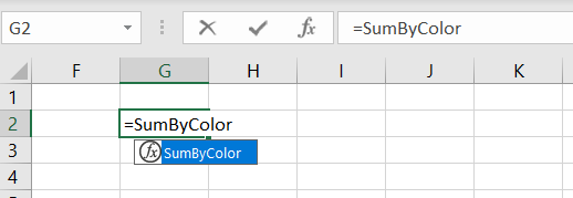
    Let’s test this out. We named our user-defined functions SumByColor so we should be able to see the function now if we enter it into a cell:
    User-Defined-Functions-Sum-Based-On-Colors-Excel

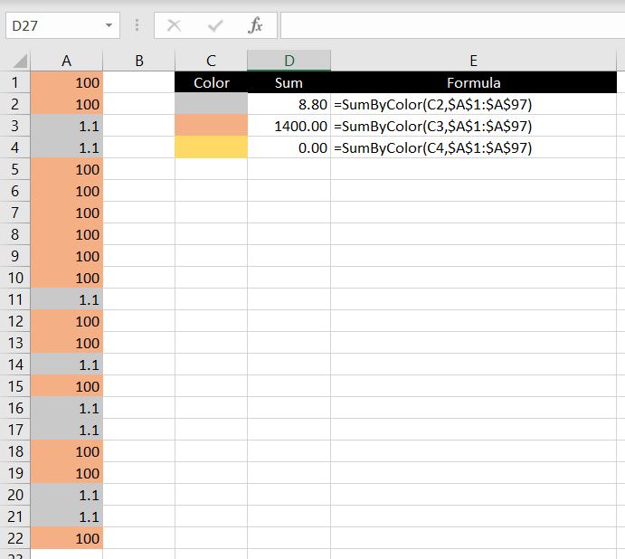
    There are two fields required: 1) colorcell and 2) cellrange:
    Sum-Based-On-Cell-Colors-Excel

    =SumByColor(C2,$A$1:$A$97)

    For each formula, we first reference the cell on the left (in the first formula: C2). This tells the function what color we are looking for. Not that we need to know but Excel looks at the color of this cell and stores the color index as WhatColor. And then Excel loops through each cell in range A1:A97. For each cell which has color matching WhatColor, the value gets added onto a variable called x. And at the end of the loop, the function returns the value of x.

    Note that the “If IsNumeric(coloredcell) = True” is important because otherwise we could be asking Excel to do an addition with non-numerical values, in which case Excel would return #VALUE. But with this condition added to the IF statement, if Excel recognizes that the value is not numerical (even if the color matches), it will skip over this value:

    Sum-Non-Numerical-Values-Excel

    COUNT Number of Cells With A Particular Color

    Next we will look at how to create a user-defined function that can count the number of cells that are filled with a particular color. Again, first thing to do would be to make sure our Excel file is macro-enabled.

    Secondly we will need to think of a name for our function. In this case, we will call our function: CountByColor. Essentially you can give your function whatever name you want (except one that is already used by a built-in function in Excel) but it is good practice to choose a name that actually makes sense to you and to everyone who will be using your Excel file.

    Similar to calculating the sum of values based on the cells’ colors, we need the exact same variables/inputs for this function:

    1. The cell that has the color which we want to reference for this function: colorcell
    2. The range of cells which the function will check if the cell color is colorcell (from above): cellrange
    Public Function CountByColor(colorcell, cellrange) As Integer

    WhatColor = colorcell.Interior.Color
    x = 0

    For Each coloredcell In cellrange
    If coloredcell.Interior.Color = WhatColor Then
    x = x + 1
    End If
    Next coloredcell

    CountByColor = x

    End Function

    Now let’s explain the codes step by step:

    1. First off, we need to let this function know the color it is looking for in the range of cells. And that is what the first variable or field is for: colorcell. Whatever color this cell is filled with, this function will match every cell in the second variable against this color. And we create a variable WhatColor to store this color index:

      WhatColor = colorcell.Interior.Color
    2. Next we create another variable called x – this variable will keep adding one to itself if the cell color matches with WhatColor. At the start of this function, we will set:

      x = 0

      This is because at this point, we haven’t checked any cell in cellrange against WhatColor yet.
    3. The next step is to run a loop. The loop will go through each cell in the cellrange specified in the function:

      For Each coloredcell In cellrange

      Note that the variable coloredcell can really be called anything. It’s just another variable we’re creating for this loop.
    4. For each cell in the cellrange, we want to check if the cell color matches WhatColor. If it does, then we will add one each time to x:

      If coloredcell.Interior.Color = WhatColor Then
      x = x + 1
      End If


      Optional: Note that in the SumByColor function, we had the additional check to make sure the cell value is numerical. We didn’t do that in this case since we are not adding any values together. But theoretically, we could add more conditions. E.g. we could make sure the cell is not blank by adding:

      And Len(coloredcell)>0

      In which case, the If statement becomes:

      If coloredcell.Interior.Color = WhatColor And Len(coloredcell) > 0 Then
    5. Once all the cells in cellrange is looped through, the final x will be the total number of cells that are filled with WhatColor. And this is what we want the function to return:

      CountByColor = x

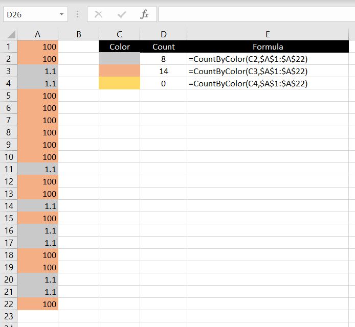
    Let’s test this out. You should now be able to see a CountByColor function:
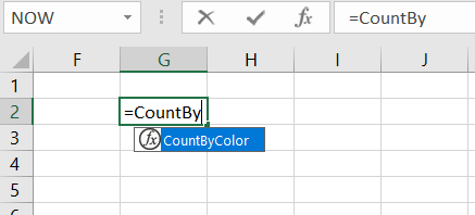
    User-Defined-Functions-Count-Based-On-Colors-Excel

    There are two fields required:

    Count-Based-On-Cell-Colors-Excel

    We first reference the cell on the left (in the first formula: C2). This tells the function what color we are looking for. Excel then stores this color index as WhatColor and then it loops through each cell in range A1:A22. For each cell which has color matching WhatColor, the variable x adds one to itself. And at the end of the loop, the function returns the value of x.

    As mentioned above, we could add more conditions depending on what we need. For example besides from the color of the cell, we could also test whether the value is numerical, or we could test whether the value is over 1000.

    What To Be Mindful Of…

    Before we end the article, let’s go through what we need to be mindful of with these two user-defined functions above because there are key two limitations:

    1) When Does The Function Recalculate Itself?

    One thing to keep in mind is whether the function recalculates itself automatically and when. In Excel, if in a function you reference another cell or range of cells and let’s say the value in those referenced cell(s) changes, the value from your function will update itself automatically.

    Rest assured this is the same with the user-defined functions we just created. However from Excel’s perspective, changing a background color of a cell is not the same as updating/changing a value in a cell. Simply put, changing a cell color is not a catalyst for Excel to recalculate its functions and formulas. This means if you add a number into a cell and then change the color of the cell, the two user-defined functions will not pick them up (at least not until a value is updated somewhere in the worksheet that will trigger Excel to recalculate all its functions and formulas).

    Workaround:

    Instead of entering a value into the cell and then changing the color of the cell, do it the other way around. You will need to first change the color of the cell and then update value in it. Simply put, it is the updating of the value that triggers Excel to recalculate all the functions and formulas. So by updating the value after changing the cell color, the user-defined functions will be updated.

    2) This Does Not Work With Conditional Formatting

    Unfortunately this just doesn’t work with conditional formatting. To illustrate this, we created another user-defined function: WhatColorCell. This function checks the color of a particular cell and returns the color index:

    Public Function WhatColorCell(checkcolor) As Double

    CellColor= checkcolor.Interior.Color
    WhatColorCell = CellColor

    End Function

    In the examples below, we used this function on three different cells 1) the first one is filled with red, 2) the second has conditional formatting such that if the cell value is over 200, it will be formatted as red and 3) the cell has no color filled at all:
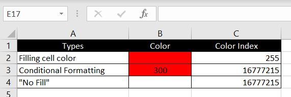
    Conditional-Formatting-Color-Cell-Excel

    As we can see, even with conditional formatting, the color index returned is the same for 2 & 3. From Excel’s perspective, a conditionally formatted cell has the same color index as a cell with no filled color. That is, provided of course the conditional formatted cell was not previously filled with a color.

    We hope everyone finds this article helpful. If you have any questions regarding this article or if you have any suggestions on how we can change it and what we can add, please leave a comment below!


  • How To Use Radio Buttons In Excel

    How To Use Radio Buttons In Excel

    In this article we will go through how to insert radio buttons in Excel, how they work and how to use the results. In another article – How To Insert Check Boxes In Excel, we went through the key differences between check boxes and radio buttons. In that article, we also did a walkthrough on how check boxes work in Excel. This time, we will go through radio buttons. In short, the key distinguishing features of radio buttons are that with radio buttons:

    • Only one button can be selected at a time
    • One button must be selected at any given time. That is, we cannot deselect all the buttons – there is one way to do this

    Radio-Buttons-Excel

    How To Insert Radio Buttons

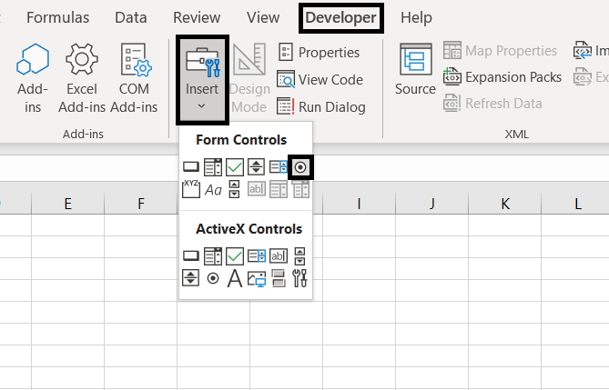
    Similar to check boxes, we will first need to make sure Developer tab is enabled and the Excel file is saved in a macro-enabled format. Once we do, we can go to Developer tab at the top > Insert > Option button:

    Insert-Radio-Buttons-Excel

    We can then click on anywhere within the spreadsheet and a radio button will be inserted:

    Radio-Buttons-Inserted-Excel

    Formatting Radio Buttons In Excel

    Before we keep going, let’s go through some basic formatting with radio buttons.

    First of all, if we click on the button, we will be selecting the button or choosing the option. To move it around or edit the button, we need to either:

    • Hold the CTRL key and click on the button
    • Right-click on the button

    After we see the box around the button, we can move it around or resize it. We could also copy and paste to create more buttons rather than going to Developer > Insert > Options Buttons every time.

    To edit the text next to the button, right-click the button and select Edit Text.

    Linking Buttons To A Cell

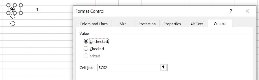
    The next step would be to link the buttons to a cell. Why do we need to do this? Because by linking the buttons to a cell, the relevant button selection will then be converted into a value in that cell. And of course with the value in that cell, we can then apply formulas or do conditional formatting with it.

    To link the buttons to a cell:

    • Right-click on the button
    • Select Format Control
    • In the Cell Link field, select the cell you want to link the button to:

      Linking-Cells-Buttons-Excel

    Unlike check boxes where we need to link each check box manually to a different cell, because we can only select one radio button at a time, we only need to link the cell once. Also because of this difference between radio buttons and check boxes, the returned values from radio buttons are numbers whereas each check box returns a TRUE or FALSE result. With radio buttons, it depends on how many buttons have been inserted. Say there are 5 buttons and if the first one is selected, 1 will be returned as the value in the linked cell. If the third button is selected, 3 will be returned as the value in the linked cell:

    Radio-buttons-linked-cell-Excel

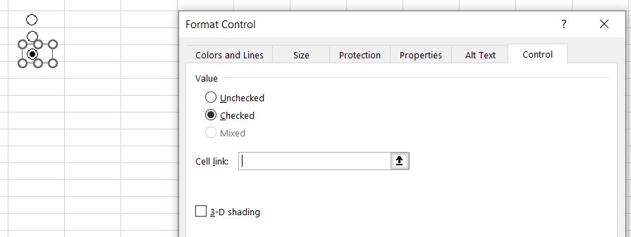
    How To Deselect All Buttons

    At first glance it would seem like you cannot deselect all the radio buttons because by clicking on an already selected button, it…just stays selected, unlike a check box. But there is a way to deselect all buttons:

    • Right-click the selected button
    • Select Format Control
    • In the Value section, make sure the button is unchecked:

      Deselect-All-Buttons-Excel

    And all buttons will be unchecked:

    All-Radio-Buttons-Deselected-Excel

    How To Use The Selection Result

    The next step is to look at what we can do in Excel after a button is selected. After all there is not much use if we can create buttons but not use the results. It would just become a survey that requires manually calculation and analysis.

    As an example, we exported our friend’s running log in Garmin and there’s a list of 290 running activities like below:

    Running-Activities-Excel

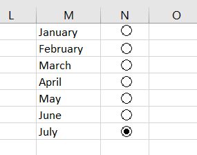
    We can then insert a few buttons, one for each month:

    Radio-Buttons-Months-Excel

    Following the same steps as above, we’ve linked the buttons to cell N1. With that, if we select the “January” button, we will see the value 1 in cell N1. If we select “May”, we will see the value 5 in cell N1. You can link the buttons to any empty cell and it doesn’t matter because we are going to hide the value by changing the font color to white.

    Because we now know that every time we select a different button, the value in cell N1 will update itself, we can now create a table and put in formulas that return different results depending on the value in cell N1:

    Selecting-Months-Excel-Buttons

    =INDEX(M1:M12,N1,1)

    We decided to use an INDEX function here. It is perfect in this situation. Whatever number is returned in N1 as a result, the INDEX function will return that row’s value in the M1:M12 array. If “July” is selected, N1 will return 7. The INDEX function will look for the 7th value in the M1:M12 range which is “July”. And once we’ve used INDEX function to identify the month, we can use various functions such as COUNTIF, SUMIF and AVERAGEIF to gather more information for the month:

    Button-results-Excel

    As we can see, depending on the month selected, the values in the table change accordingly:

    Formulas-Radio-Buttons-Excel

    Summary: we’ve set up 7 buttons – one for each month. All the buttons are linked to cell N1. With INDEX function in Q1, we can identify the month selected with the radio buttons based on value in N1. Then the rest of the formulas refer to the value in Q1.

    How To Group Buttons Together

    So far we’ve only looked at situations where only one button at be selected at a time. But is it possible to select more than one button in a worksheet? Perhaps by assigning radio buttons together into groups so that in each group we could make a separate selection.

    To do that, we will need to follow the steps below:

    1. In the Developer tab, Insert > Group Box

      Developer-Group-Excel
    2. Draw a Group Box on the worksheet
    3. In the Develop tab, Insert > Option Button
    4. Create two or more buttons
    5. Put all the buttons inside the Group Box
    6. Select all buttons and the Group box by holding CTRL key and left-clicking
    7. Right-click > Group > Group

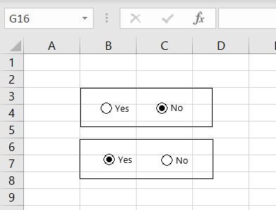
    Follow the same process above to create more groups of buttons. With buttons being grouped separately, each set of buttons can be selected independently from buttons in other groups:

    Multiple-Buttons-Selected-Excel

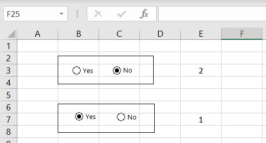
    And of course we can link each group of buttons to a cell. In the example below, we linked the first group of buttons to cell E3 and the second group to cell E7:

    Multiple-Groups-Buttons-Linked-Cells-Excel

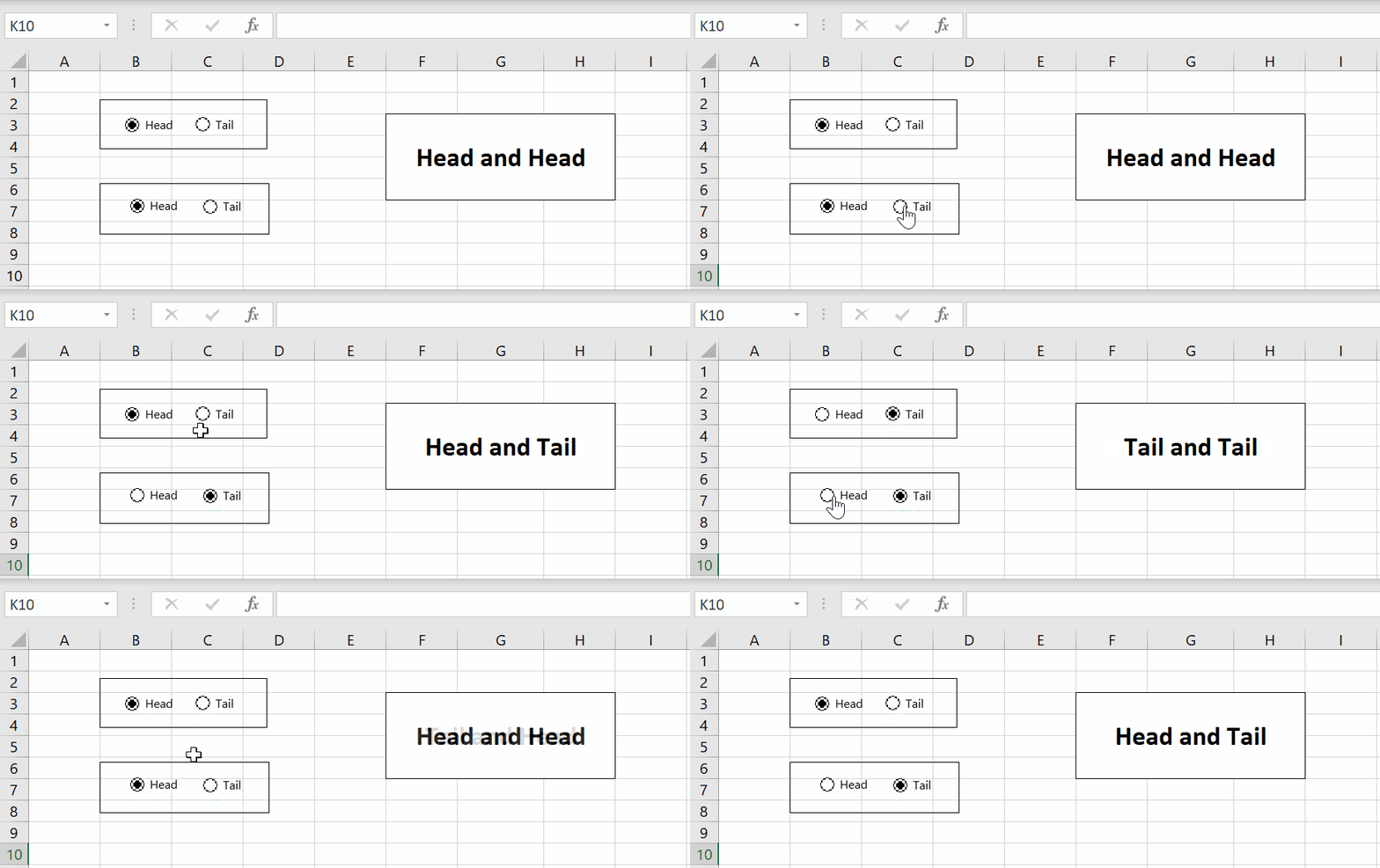
    Here’s an example below:

    Multiple-Buttons-results-Excel

    =IF(E3=1,”Head”, “Tail”)&” and “&IF(E7=1, “Head”, “Tail”)

    If there’s anything you would like us to add to this article, please leave a comment below. We hope you now understand how radio buttons work in Excel, how to insert them and format them.

  • SUMIF – SUM IF Condition is Met

    SUMIF – SUM IF Condition is Met

    Similar to the COUNTIF function, SUMIF is also one of the most fundamental functions to use in Excel when it comes to reporting and data analysis. In this article, we will go through how this function works and also explain why values may not be adding up correctly. We will also apply multiple conditions in SUMIFS function. And we will set conditions with greater than/less than or equal to.

    SUMIF – How It Works

    Let’s first go through the basics of how the SUMIF function works. And as obvious as it sounds, we should start by explaining what the function does. SUMIF is a:

    • Built-in Excel function that allows users to calculate the sum of certain values if a condition is met. For SUMIF, there are three inputs/variables requires for the function: range, criteria, and [sum_range]:
      • Simply put, Excel would add up values in the array (sum_range) if values in the range meets the criteria

    =SUMIF(range, criteria, [sum_range])

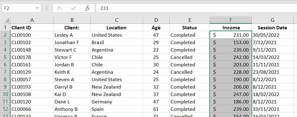
    Let’s use data below as an example:

    Excel-SUMIF-Data

    With SUMIF function, we could do more insightful analysis such as getting total income based on location or total income for each year. We could basically separate data into groups. For example we could look at total income by age brackets of the clients.

    SUMIF-Basic-Example-Excel

    =SUMIF($C1:$C196,I2,$F1:$F196)

    In this example, we are adding income (sum_range – Column F) together if the location (range – Column C) matches our criteria (I2). In Cell I2, we have “United States”. Hence for every row where we have “United States” in Column C, Excel will add the income in Column F because the condition is met. And similarly for Brazil, Argentina and other locations.

    The good thing about SUMIF function is that it is not limited to the range column being on the left of the sum_range column. In the example above, we could easily have swapped Column C and Column F and SUMIF could still perform the exact same calculation for us.

    Numbers Not Adding Up Correctly? Important!

    Are values not adding up correctly? This, for obvious reason, is worse than getting an error. Why? Because it is not always obvious that we’ve made a mistake! This is why it is important to make sure we enter values into SUMIF function correctly, otherwise we could be getting an incorrect answer without even knowing it.

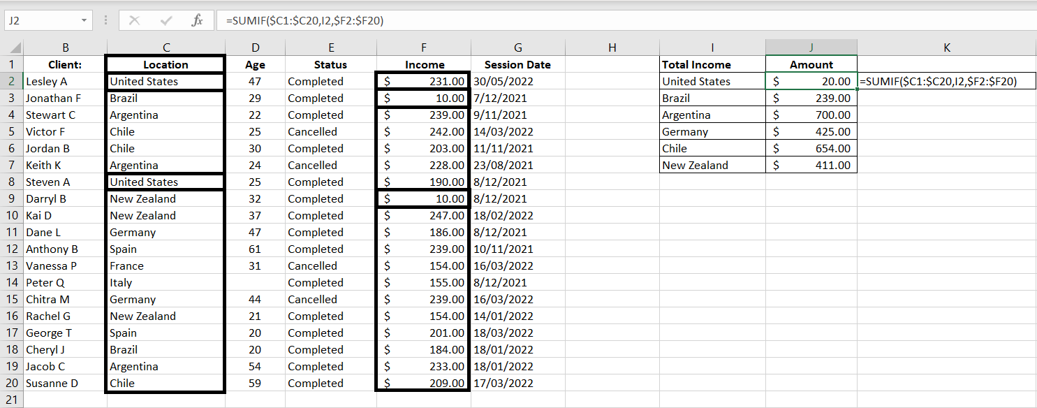
    With the SUMIF function, there are two arrays we need to enter: 1) range and 2) sum_range. It is very important that the two are aligned. Especially because of headings, it is easy to make a mistake and start one array in row one and the other in row 2. To clearly illustrate the problem and how the function works, we have changed the numbers and made the table smaller to make this more obvious:

    SUMIF-Numbers-Not-Adding-Up-Excel

    =SUMIF($C1:$C20,I2,$F2:$F20)

    Notice that the range starts with Row 1 (C1) and sum_range starts with Row 2 (F2). Because of that, the corresponding rows do not match up anymore. From Excel’s perspective, the second and eighth rows in range C1:C20 are “United States”, hence it will return the second and eighth rows in sum_range F2:F20. But the second and eighth rows in F2:F20 are $10 and $10. Hence the SUMIF function returns $20 as the result.

    SUMIF with Dates and with Greater or Less Than

    So far we have only looked at examples where the criteria and values in range are exact matches. What if we don’t want an exact match? What if we want greater than (>) or less than (<)? Or what if we want to add up values across a certain period of time?

    Greater Than or Less Than…

    Let’s first look at how greater than and less than work in SUMIF functions. In this simple example, we will add up values in Income column if values in Age column is 1) over or equal 35 and 2) under 35:

    Excel-SUMIF-Greater-Than-Less-Than-Excel

    =SUMIF($D$2:$D$196,“>=”&35,$F$2:$F$196)

    =SUMIF($D$2:$D$196,“<“&35,$F$2:$F$196)

    Both are almost exactly the same except for the criteria. After all, both are looking at the same Age Column and the Income Column. In the first function, we want greater than or equal which is “>=”. And to connect that with 35, we just need to add a & in between.

    Similarly with the second formula, we want a less than which is “<“. And we connect it with &35. In this case we don’t want a “less than or equal to” because the “equal to” would overlap with the first “Over or equal 35” formula.

    Note: there are in fact some blank fields in the Age column but Excel would ignore them. To Excel, that means a blank cell is not the same as 0. With a “less than 35” condition, a blank cell is not considered meeting the condition. And in fact that would be perfect in our scenario, Column D is an Age column. A blank cell would more accurately be considered as “unknown“, not 0.

    SUMIF with Dates

    Using very similar logic, we can add up values if the dates fall within a particular range. Here we want to add up values in Income column if Session Date is prior to 2022:

    SUMIF-Dates-Excel

    =SUMIF($G$2:$G$196,“<“&DATE(2022,1,1),$F$2:$F$196)

    The range we are comparing the criteria with is G2:G196. The criteria is that the value in this range must be less than “<“ 01/01/2022 which is represented by DATE(2022, 1, 1) and we again connect the two with &. We could simply put it in a regular date format with quotation marks, e.g. “01/01/2022”. However because different countries could use different date formats (e.g. mm/dd/yyyy or dd/mm/yyyy), it will be less confusing to just use the DATE(year, month, date) function.

    Note: the good thing with SUMIF function with dates is that it knows to ignore blank cells in the range. That is if a cell is blank in G2:G196, it will NOT be considered as a condition met.

    Tip: always check your work. If the SUMIF function that is greater than or equal to a date and another SUMIF function that is less than that same date do not add up to the total, then you would know that there’s probably a field missing in the session date.

    SUMIFS – Multiple Conditions

    What if we want to add multiple conditions into SUMIF function? Well luckily there is a SUMIFS function. It is literally just a SUMIF but with multiple conditions. The order we enter our variables changes slightly. With SUMIFS, it is:

    = SUMIFS(sum_range, criteria_range1, criteria1, [critieria_range2, criteria2]…)

    Notice that there is no square bracket around sum_range now. This means sum_range is now a mandatory field. The first set of range and criteria is also mandatory. But conditions 2, 3, 4…are optional. Excel-SUMIFS-function-multiple conditions

    =SUMIFS($F$2:$F$196,$C$2:$C$196,I2,$E2:$E196,J2)

    =SUMIFS($F$2:$F$196,$D$2:$D$196,”>”&45,$E2:$E$196,J3)

    The easiest way to visualize this is first we tell the function the range of cells which has the values we would like to add up (F2:F196). After that, we put in each set of criteria_range and the criteria:

    • In the first example, for Column C (Location), we are looking for “United States” as the criteria (Cell I2) and also in Column E (Status), we are looking for “Completed” as the criteria (Cell J2)
    • In the second formula, for Column D (Age), we are looking for values greater than 45 as the criteria and also in Column E (Status), we are looking for “Cancelled” as the criteria (Cell J3)

    Sum_Range Can Be Optional?

    Ever noticed that in the SUMIF function, sum_range is in square bracket? This would of course mean that this field is an optional input. The function can still work with or without this variable. Strange but it works.

    If the sum_range is blank, Excel will add up values in range field. That is, of course only if values in range are numerical values. We will show two examples below:

    1) Numerical Values

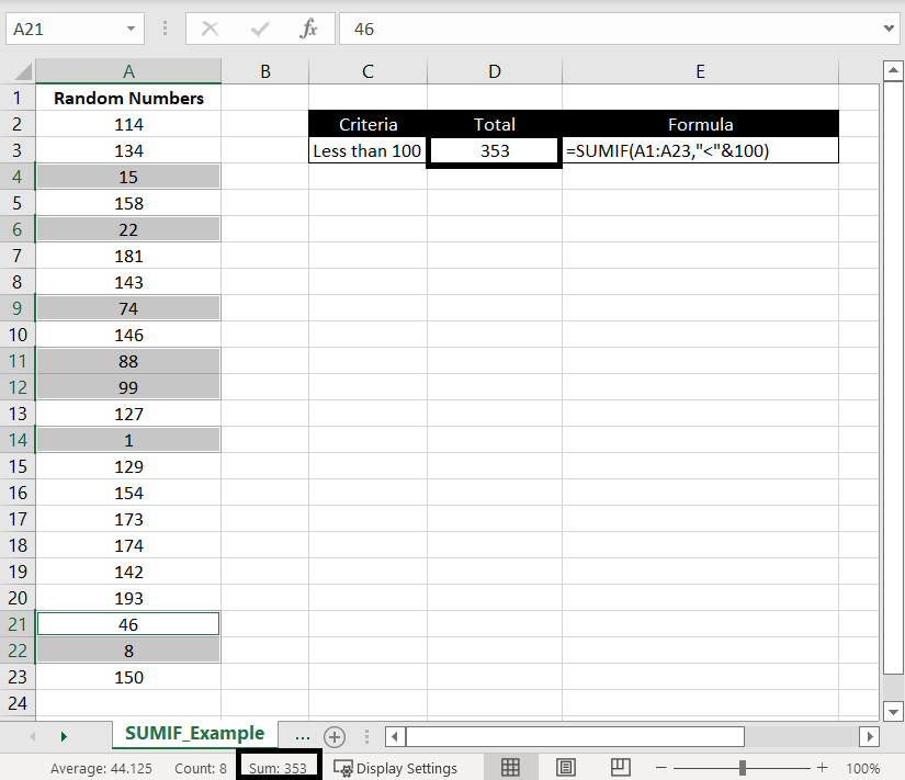
    Here’s a list of random number between 0 to 200 – randomly generated by RANDBETWEEN. In this example, we will add up the numbers if they are less than 100:

    SUMIF-Example-No-Sum_Range-Excel

    =SUMIF(A1:A23,”<“&100)

    We highlighted cells with values less than 100 and we can see at the bottom the “Sum: 353” matches the SUMIF result. This shows that while the criteria is being matched against the range, values in the range would be added up.

    2) Non-Numerical Values

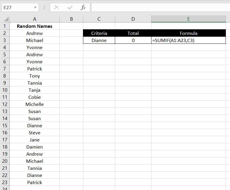
    Here we are doing a SUMIF in range A1:A23 and the criteria is “Dianne”:

    SUMIF-No-Sum_Range-Names-Example-Excel

    =SUMIF(A1:A23,C3)

    Again no alert pop up appeared. Excel will happily calculate the function for us because sum_range is only an optional field. But as expected, because names are non-numerical values, there is nothing to add up. Hence the SUMIF function returns a 0.

    We hope you now have a good understanding of how SUMIF works in Excel. If you need any further clarification or if you feel that we’ve missed anything, please leave a comment below.

  • User-Defined Functions – Writing Your Own Functions in Excel

    User-Defined Functions – Writing Your Own Functions in Excel

    There are over 500 built-in functions in Excel but yet you may have trouble finding one that suits your need. Are there calculations that you do on a regular basis over and over again? And you are tired of typing in that same formula in again and again every time. You can save time by writing your very own user-defined functions in Excel.

    Before we start, we need to make sure the Developer tab is enabled in Excel. If you don’t see a Developer tab at the top, it’s simple – have a look at How To Enable Macro/Visual Basic for Application (VBA):

    Developer-tab-enabled-Excel

    If you can see the Developer tab, then let’s get started! We will first go through a simple example of creating a function that calculates the area of a circle. And then we will go through another example which is more complex and uses a loop.

    Creating Your Very Own Functions

    1. Open Visual Basics

    You can open Visual Basics by going to Developer Tab > Visual Basics:

    Open-vba-developer-tab-excel

    Or you can press Alt + F11.

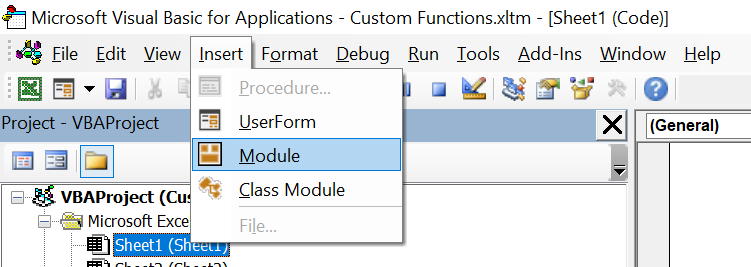
    2. Create a New Module

    At the top, click on Insert > Module:

    Create-new-module-vba-excel

    3. Name of Function and Required Field(s)

    3.1. Unique Name for the Function

    Now it’s time to think of a unique name for the function and what variables or fields should be required. It is best practice to give the function a name that is relevant to its purpose. For example, it’ll be very confusing to others who use the spreadsheet if you name the function “Bob”. And it’ll be confusing for yourself. A few months later you might come back and wonder what the function “Bob” is supposed to calculate. In this example we will create a user-defined function that calculates the area of a circle so we will call the function “AreaOfCircle”.

    You also want the name to be unique. Because Excel already has over 500 built-in functions, you won’t want one that is already used by Excel. In fact, if you do, your user-defined functions will not work. Excel’s built-in existing functions will take place over your user-defined functions.

    3.2. Variables and Fields

    Technically not every function requires variables. It probably won’t be of much use but you can create a function that returns a constant value every time. For example you can leave the variables blank and have the function AreaOfCircle = 2 in the module. In which case, AreaOfCircle() will always return 2. But for example if we want to calculate area of a rectangle then the variables will be length and width.

    In this scenario, what variables are required in order to calculate the area of a circle? Since A = πr2, the only variable is r – the radius. In the empty module, enter the following:

    Public Function Name of your Function (variable1, variable 2…)

    End Function

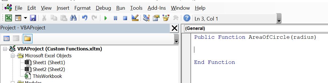
    And in our case:

    Creating-UDF-Excel

    Public Function AreaOfCircle (radius)

    End Function

    4. Write Your Formula and Calculation

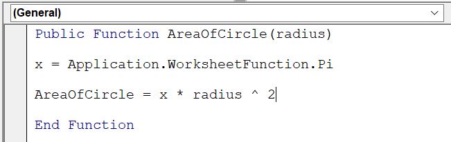
    This is of course the crux of the function. What is your function? What would you like Excel to calculate for you with this new function? To stick with our example above, we want to calculate the area of a circle:

    Area-of-circle-UDF-function-Excel

    We first set a new article x to be the value of Pi. And then we set AreaOfCircle to equal x * radius ^ 2 which is equivalent to A = πr2. In this case we set x as Pi.

    Public Function AreaOfCircle (radius)

    x = Application.WorksheetFunction.Pi

    AreaOfCircle = x * radius ^ 2

    End Function

    5. Let’s Check Our Work!

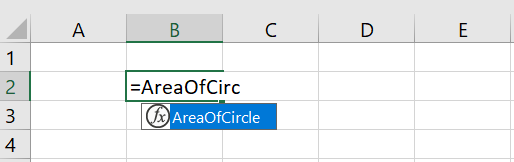
    Go back to our Excel sheet. Click on any cell and start typing “=” and the name of your function. You should be able to see it:

    Checking-UDF-Excel-Functions

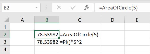
    Once you see that your function is there, let’s check the calculation. The easiest way is to use this function in one cell and then put in the exact same formula in the cell underneath it manually with the same variable(s). Check out below:

    Testing-UDF-function-Excel

    The results are the same which is good. Test out a few more variables to make sure the function is working as intended.

    6. (Optional) Setting Variables Using IF Statements

    Now that our function is working, is there a way to improve it? This part is optional. Depending on what your function is, in most cases there should be parameters around what your variables could be. For example in some cases, the variables should only be integers. And in the case of a circle, the radius should only be a positive number. It can be a decimal but it certainly does not make sense to have a negative radius.

    To do this:

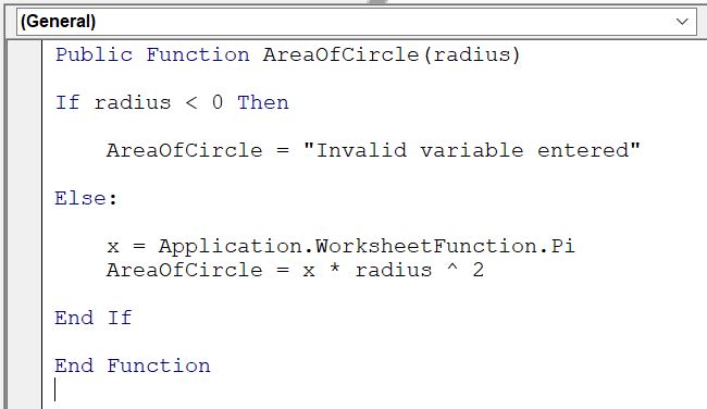
    Before defining the AreaOfCircle function, add an IF function. If the radius variable entered is less than 0, the function will return “Invalid variable entered”. In all other situations, calculate the area of circle.

    Public Function AreaOfCircle(radius)

    If radius < 0 Then

    AreaOfCircle = “Invalid variable entered”

    Else:

    x = Application.WorksheetFunction.Pi
    AreaOfCircle = x * radius ^ 2

    End If

    End Function

    Invalid-Variable-UDF-function-module-Excel

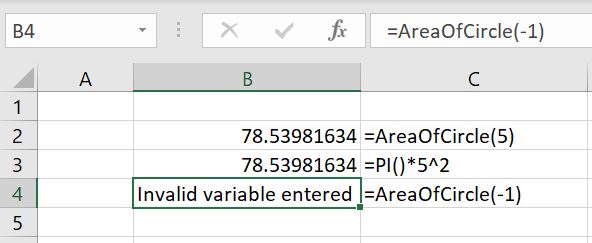
    Invalid-Variable-UDF-function-Excel

    In these cases, notifying the user an invalid variable was entered would most likely be more useful than actually calculating the area of circle with a negative 1 radius.

    Now let’s move onto a more complex example which involves a loop in the user-defined function

    Creating a User-Defined Function with Loop

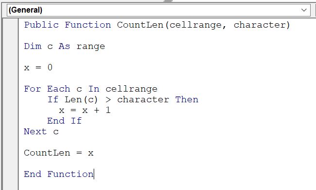
    When we were writing the article for COUNT functions, it got us wondering if, given a specified range of cells, there was a way to count the number of cells containing data that has more than x number of characters inside. Well let’s write our own:

    Public Function CountLen(cellrange, character)

    Dim c As range

    x = 0

    For Each c In cellrange

    If Len(c) > character Then

    x = x + 1

    End If

    Next c

    CountLen = x

    End Function

    UDF-function-with-loop-Excel

    To put this into words:

    • We’ve called this new function “CountLen” and there are two variables required by the user every time: 1) the range of cells to count in (cellrange) 2) how many characters should be in the cell in order for the function to count the cell as meeting the condition (character)
    • First we create a new variable x and we set it as 0 at first. And for each cell in the range of cells specified (cellrange), if the number of character is greater than what we’ve specified in the second variable (character) then Excel will add 1 to x every time. After all the cells have been looped through, CountLen will return the value of x.

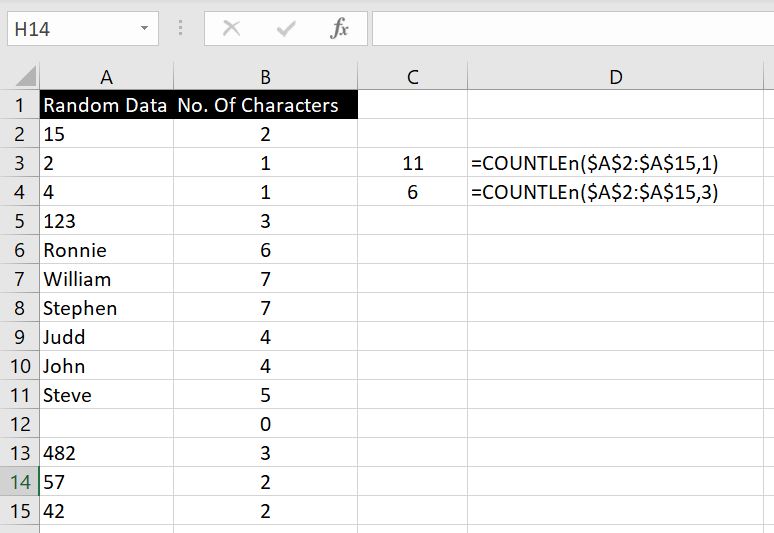
    Here’s an example below. In A2:A15, we’ve entered a bunch of random data. Let’s test this out with different variables to check if our function is working. Note that in the function, we’ve decided to set the function to check if the number of characters in each cell is greater than second variable specified, not greater than or equal to. Hence if we set the second variable as 2, Excel will only count if the number of characters is 3 or more:

    Testing-UDF-Loop-Function-Excel

    To check our results, we created Column B which counts the number of characters in corresponding cell in Column A with the LEN function. There are 11 cells in A2:A15 that have more than one character in them, and there are 6 cells in A2:A15 that have more than 3 characters in them.

    Are there any user-defined functions you need help with and want us to go through? Let us know in the comment below and we will keep add to our article to make it more complete.

  • How To Enable Macro/Visual Basic for Application (VBA)

    How To Enable Macro/Visual Basic for Application (VBA)

    To enable Macro/Visual Basic for Application (VBA) in Excel, there are two steps. Before we start, let’s talk about what Macro and VBA are about.

    Macro is a recording tool in Excel – we press a button to “start recording”, we then do a series of activities/processes and at the end we press a button to “end recording”. Excel records that series of activities/processes so that with a click of a button, Excel will repeat those specific steps for us.

    VBA (Visual Basic for Application) is very similar. Except, instead of recording the series of steps, we have to write them as lines of codes in modules. We can create user forms, automate a series of steps, create reports, send emails out and a lot more. It is important to note that Macro is really part of VBA. Once the series of activities/steps are recorded, the Macro is essentially created into a module in VBA and we can go in to review/edit the codes.

    Tip: a simple way for anyone to start learning VBA is to record a simple Macro and then go into VBA to review the module. That way we can learn the basics of how VBA language works.

    We will not go through how to record Macro or how to use VBA in this article. They will come in later articles. Right now, let’s first go through how to set up Excel properly so that it is ready to use Macro/VBA:

    1. Enabling Developer Tab

    To enable the Developer tab:

    1. Go to File > Options
    2. Click on Customized Ribbon
    3. Under the Main area, make sure Developer is in this section and selected. If Developer is not already in the Main tab, you can find it in All Commands section and add Developer to the Main area:

    developer-tab-option

    And you will be able to see the Developer tab:

    developer-tab

    2. Save the File as Macro-Enabled Worksheet Format

    The second step is to save the file as Macro-Enabled Worksheet format:

    1. Go to File
    2. Click on Save As
    3. Select folder path
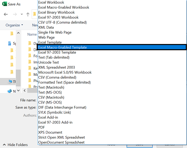
    4. Save as type: Excel Macro-Enabled Template

    macro-enabled-format

    Once that is saved, your Excel file is now in Excel Macro-Enabled format.

    And that’s it. You will now be able to see the Developer tab, record a Macro or go into Visual Basic and start inserting your own module and write some codes. If we’ve missed anything in this article, feel free to leave a comment below!