Category: Layout and Formatting

How to Freeze a Row or Column in Excel
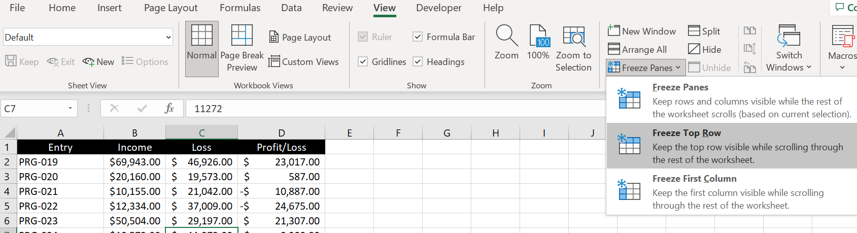
Do you want to freeze a row or column in Excel? Do you find yourself constantly having to scroll back up to the top or to the left of the table to look at the headings? For example below, freezing the top row would be very useful because without row 1, we will not know what each number in Column B, C and D refers to.

Freeze Top Row or First Column

To freeze the top row:
1. Scroll to the top
2. Go to View tab
3. Click on Freeze Panes
4. Select Freeze Top Row
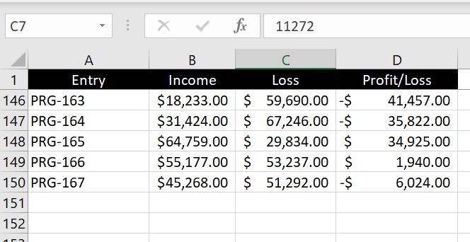
We can now scroll down and Row 1 will always be visible, making it clear what each column is:

And of course we could follow very similar steps to freeze the first column:
1. Scroll to the left
2. Go to View tab
3. Click on Freeze Panes
4. Select Freeze First Column
And now we can scroll to the right and Column A will always be visible, making it clear what each row is referring to:

Limitation: we cannot use both Freeze Top Row and Freeze First Column together. As soon as you select the other one, the first one disappears. Find out below how we can freeze both row and column.

Freeze Row and Column

There is of course a way to freeze both row and column in Excel. In fact the row and column do not have to be the top row or first column. We could freeze from Row 5 and from Column G if we wanted to. The easiest way would be to:
1. Select the cell which is in the row and column we would like to freeze
2. Go to View tab
3. Click on Freeze Panes
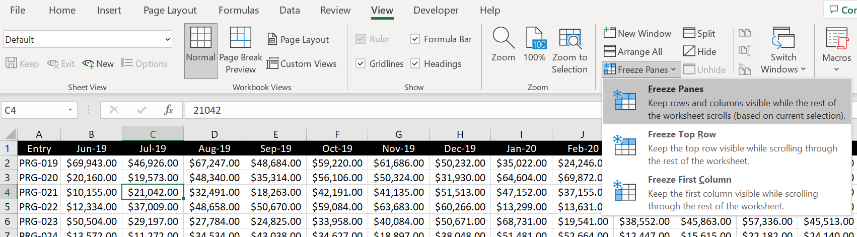
4. Select Freeze Panes
And because C4 was selected in the picture above, Row 3 and Column B will now be frozen:

Freeze Any Row OR Column

In the section above, we went through how to freeze a row and column at the same time. In this section, we will look at how to freeze any row or column and they are not necessarily the top row or first column:
1. Highlight the relevant row or column
2. Go to View tab
3. Click on Freeze Panes
4. Select Freeze Panes
And as we can see, Column G is now frozen:

Similarly we can do the same thing with any row by first highlighting the relevant row.

Unfreeze Panes

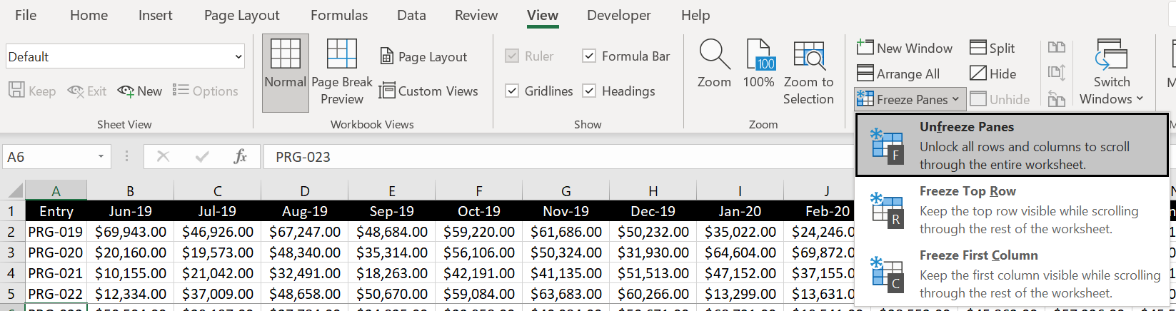
Unfreezing pane is simple. We don’t even need to highlight the relevant column or row or have the cell selected. We could do so by:
1. Go to View tab
2. Click on Freeze Panes
3. Select Unfreeze Panes
Hotkeys for Freezing (or Unfreezing) Panes

To freeze panes using hotkeys:
- ALT > W > F > Choose the following:
- F: to freeze or unfreeze pane
- R: to freeze top row
- W: to freeze first column
And we recommend using the following hotkeys along with freezing panes:
- Shift & space: highlight row
- Ctrl & space: highlight column
We hope you find this article useful. If you have any more questions regarding freezing panes in Excel, please leave a comment below and we will keep editing this article to make it more and more useful for everyone.
November 3, 2023
How to Change and Substitute Specific Text in Excel
There could be various reasons why we need to change and substitute certain text in a cell. We have touched on this previously when needed to take out certain part of a string in a cell (How to Extract Part of a Text in Cells). You could be doing this to clean up data or simply to help with reporting. Whatever reason it is, in this article we will go through two ways on how to change and replace specific text in Excel.

Find and Replace

We will first go through the more simple way of doing this. And that is to use the Find and Replace function in Excel. The hotkey for it is CTRL & H. Alternatively we can find it in the Home tab, in the Editing section > Find & Select > Replace…:

Here we could find and replace any text we would like. If no cell is selected, the “Find and Replace” will apply to everything in the worksheet. However we can have selected cells highlighted and only replace specific texts for those certain cells.

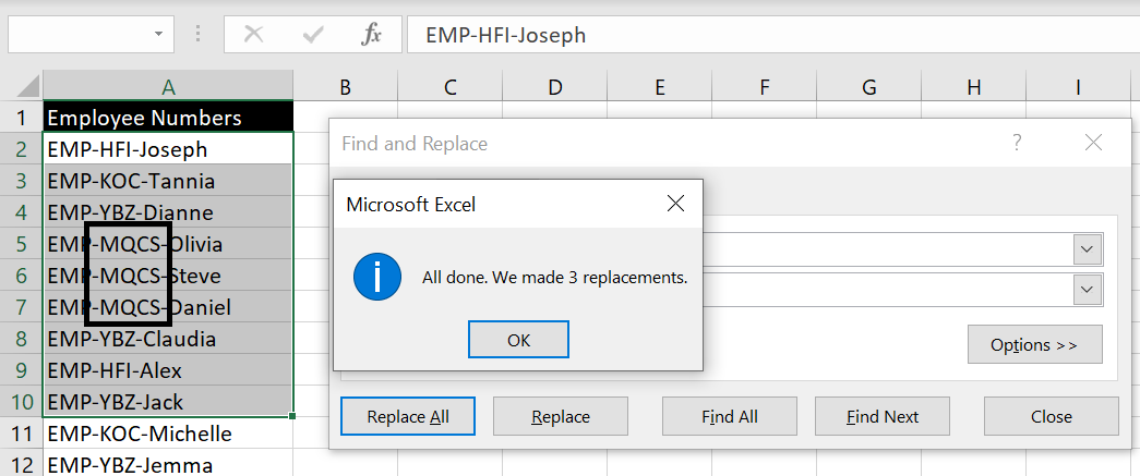
For example below, we only have A2:A10 highlighted and we will replace all “PCS” to “MQCS”:

Click “Replace All”:

Simple to use but has certain limitations:
- In a cell where the text appear in multiple instances, we cannot specify whether we only want to replace the first or second or third text. E.g. in the example above, we could not use “Find and Replace” to only replace the second dash
- Not being in a formula or function also means we cannot wrap this with another formula. And to not change the original data, we would have to copy and paste data into another location, do a “Find and Replace” and then apply another formula/function to it. That is just not the most efficient way to use Excel.
With that in mind, we will now explore another method to change and replace specific texts in Excel. This time, with a built-in Excel function.

SUBSTITUTE function

There is a built-in function in Excel called SUBSTITUTE and its purpose is to:
- Replace existing text in a string with new text
This function requires 3 mandatory inputs and 1 optional variable:
- The text or cell reference: this can also be an array in which case the results will spill into adjacent cells
- Old text: the existing text in the string to be replaced
- New text: what the old existing text should be placed with
- [Instance_num]: this is the optional input. It is the variable which allows us to choose, in cases where the existing text appears in multiple occasions, which existing text to replace in the string. By default if this is blank, all of them will be replaced.
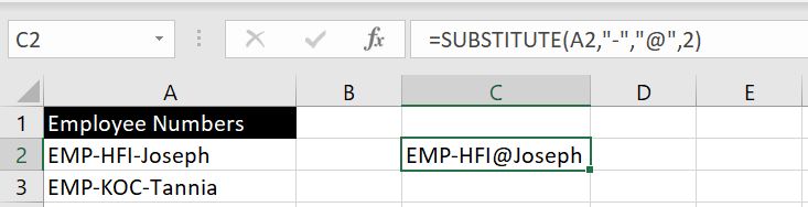
Using the above example again, with the SUBSTITUTE function, we can change and replace the second dash “-” with another character and leave the first one unchanged:

=SUBSTITUTE(A2, “-“, “@”, 2)

Here we are changing the text in cell A2. We are changing “-” to “@” and only the second instance “-” comes up. Note that if we put a number for [instance_num] that is more than the number of times the old existing text appears in the cell, Excel will just not change and replace any of them. And if we put 0 or a negative number, we will get #VALUE error.

Why Is This Useful?

There could be a number of reasons why this would be useful. One thing we can agree on is that it is definitely more flexible than “Find and Replace” or CTRL & H. With the example above, after replacing the second dash with “@”, we can now wrap the SUBSTITUTE function inside a FIND function and this will help us find where the second dash (now replaced with “@”) was:
- =FIND(“@”,SUBSTITUTE(A2,”-“,”@”,2))
And with that, we can now use the RIGHT function to extract the names of all the employees in the list:
- =RIGHT(A2,LEN(A2)-FIND(“@”,SUBSTITUTE(A2,”-“,”@”,2)))
We hope you find this article useful. If you have any more questions regarding changing and replacing certain texts in Excel, please leave a comment below and we will keep editing this article to make it more and more useful for everyone.
May 30, 2023
What You Should Use Excel For?
Microsoft Excel, the topmost spreadsheet application, offers plenty of benefits for individuals and business organizations. Being one of the most popular software, people across all industries use Excel for storing, organizing, and tracking data. With various functions and formulas, making calculations on Excel becomes highly convenient.

This guide will highlight the many uses and benefits of Microsoft Excel and show you why you should learn and be familiar with Excel.

What is Excel Used For?

Excel is mainly used for storing and calculating data. Accounting teams often use it for financial reporting and analysis. Some examples of Excel applications include editorial calendars, budgets, and balance sheets.

Thanks to its strong computational power, the spreadsheet program creates accurate financial documents. Accounting professionals use the software to calculate averages, sums, and totals. Excel helps them make sense of their business documents.

Although Excel is primarily used for accounting purposes, professionals from any field can use its formulas and features. For instance, marketers can use Excel to track different types of data.

You don’t have to spend hours counting cells or copying/pasting numbers. Excel offers quick accounting solutions to speed up data analysis and financial reporting.

Microsoft Excel allows you to analyze data and help in decision-making processes. It is an affordable and efficient solution, whether you use Excel to manage your personal or business expenses and databases.

Top Reasons for Using Excel

Here are some of the best reasons for using Microsoft Excel.

Data Analysis and Reporting

One of the best benefits of Excel is robust data analysis and reporting. Using Excel spreadsheets allows you to calculate large amounts of data with efficient sorting, filtering, and search tools. Search tools can narrow down the criteria that will help your decisions.

Combine all these tools with graphs and pivot tables and get all the necessary information. The software is scalable, and you can easily use it at home or at work.

500+ Features

This powerful software has more than 500 built-in functions that you can use for performing specific calculations. For example, Goal Seek is an in-built function in Advanced Excel Functions. This feature allows users to get their desired output when changing assumptions. This process depends on the trial-and-error method for getting results. And even if you find that the 500+ built-in functions don’t serve your need, you can write your very own user-defined function.

Some other essential features in Excel include:
- Pivot Tables
- Paste Special
- Conditional Formatting
- Add Multiple Rows
- Absolute References
- Power Query
- Extend formula across/down
- Flash Fill
- Print Optimization
- Index-Match
- Filters
VBA/Macro Coding

VBA or Visual Basic Application is a subset of the powerful Visual Basic programming language. It comes with most Office applications. While VBA helps you automate processes between and within Office applications, it is not necessary to be familiar with computer programming or VBA code if the Macro Recorder does what you want.

The macro recorder records all the steps in VBA or Visual Basic for Applications code. These steps include typing numbers or text, clicking commands on the menu or ribbon, formatting cells/rows/columns, and importing data from an external source.

Import and Export Data

Another important reason for using Excel is that it imports and exports several file types other than the standard XLSX format. Excel is compatible with many different systems. When users share data between other programs, such as a database, you may need to save data as a different file type. Using Excel as your source, importing financial data for annual or monthly periods becomes super easy.

Benefits of Using Microsoft Excel

This software is widely popular for finance and accounting purposes because it is easy to use. Excel has various front-end and back-end functions. For example, it can produce dashboard summaries and reports on the front end. On the back end, it stores and retrieves data for calculations.

Excel allows users to draw actionable conclusions from data. This reason alone is why entrepreneurs and financial professionals master this program to benefit from its features.

Here are some benefits of using Excel.

Effective and Easy Analysis

The efficient analytical tools of Excel allow users to analyze large amounts of data. That helps users discover patterns and trends that influence decisions. Thanks to the program’s graphing capabilities, you can quickly summarize data and organize it in a visually appealing manner.

All the essential types of charts you need for presenting data are already there. With a single click, you can insert a table that fits your data. The software would also ‘recommend’ a chart for you.

Collaboration

The launch of the Excel Web App made it possible for users to work on spreadsheets with others. This functionality allows users to streamline their processes. It also gives more opportunities to ‘brainstorm’ sessions using large data sets.

Thanks to these collaboration capabilities, you can use Excel Worksheets anywhere. You are no longer tied to your desk. That’s an ideal solution for business people on the go.

Excel iPad and Mobile Apps

Smartphones and tablets bring more convenience to our lives. Installing the Excel app on your device can open new possibilities. Now, you can take your worksheets to any meeting. Whether you visit a client or want to calculate finances from your couch, the spreadsheets are immediately available on your tablet or phone.

Data Transformation

You must deal with messy (unorganized) data in many situations. You can’t use this data without ‘cleaning’ or transforming it. This entire process can waste significant time and is also a tedious process.

The efficient ‘power query’ is a data cleaning and transformation engine that can load data from multiple sources. The engine transforms it and loads it back to the worksheet. This powerful data automation tool allows users to import data through external sources, such as CSV files, Text files, and the Web.

Bottom Line

Most businesses and organizations use Excel for handling statistics, data, and finances. Entrepreneurs and companies also organize, calculate, and evaluate quantitative data. These features make Excel a robust data analysis and decision-making program.
October 9, 2022
How To Identify Duplicates in Excel
What is a simple way to identify duplicates in Excel? In this article, we will go through two ways of doing that: using Conditional Formatting and COUNTIF function. And at the end we will look at how we can find the total number of unique values in a list.

Finding Duplicates with Conditional Formatting

The easiest way to finding duplicates in a column is to use conditional formatting:
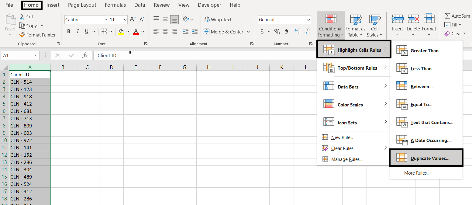
1. Highlight the column
2. Go to Conditional Formatting > Highlight Cells Rules > Duplicate Values
3. Select the formatting we want for cells that contain duplicates
4. Click OK
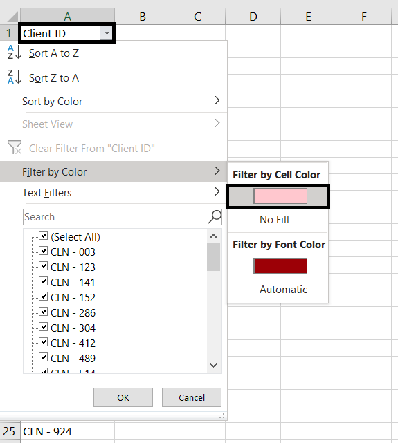
After conditional formatting is applied, we can add Filter to the column and filter by cell color:

And then we can do the cleaning up we need. We can start from the top and delete each duplicate row. But before doing so, we suggest sorting the data in order first. You can do that by going to the Home tab > Editing section > Sort & Filter > Sort A to Z:

Why do we need to do this? We want to sort the list in order first so then we can group each set of duplicates together. This is not a mandatory step but it does make it very clear how many duplicates there are for each item and hence gives us an indication on how many duplicated row we will need to remove for each.

Note: when deleting duplicates, do not delete more than one row at a time because we only want to delete the duplicated cell. The idea is when we delete/clear one cell, because there will be no more duplicate (assuming there is only one duplicate), the conditional formatting for the second cell will disappear.

Finding Duplicates using COUNTIF function

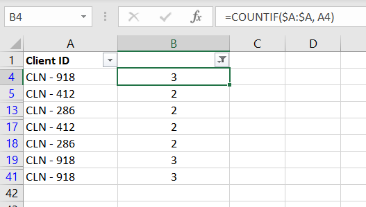
Conditional formatting certainly helps with identifying the duplicates but it does not tell us how many duplicates there are for each cell. This is something the COUNTIF function can do:

=COUNTIF($A:$A, A2)

Because we are counting that item which is inside the list itself, the COUNTIF function will not return a number lower than 1. So if we want to precisely calculate how many duplicates there are for a particular value, we can add a “- 1” at the end of the formula. For example above: “=COUNTIF($A:$A, A2) – 1”. Afterwards we could apply Filter and filter out values that have no duplicates:

Counting Unique Values

Above is the most common method we use to identify duplicates. To then count the number of unique values, we usually do one of the following:

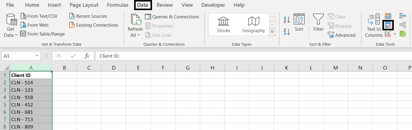
Copy the column and paste it on another sheet. Having the column highlighted, go to Data tab > select Remove Duplicates:

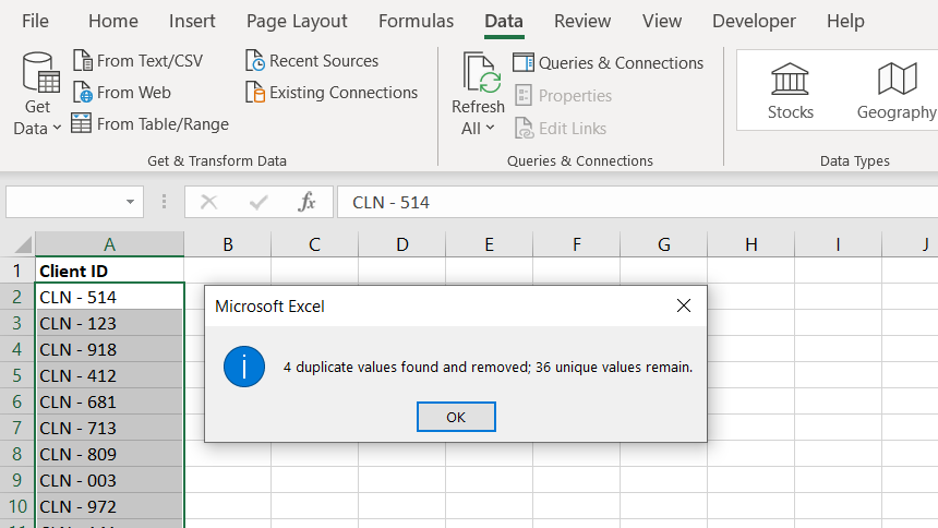
And Excel will tell us how many unique values there are in the list. We can see below Excel has very cleverly excluded the heading of the column so we know the 36 does not include the heading.

Have we missed anything on this topic? If you find that we have missed anything, or if you have any questions, want us to include anything else into this article or need clarification on anything here, please let a comment below! We want to keep improving our content so it is useful for everyone.
September 12, 2021
Why Is Excel Showing the Formula Instead of the Result?
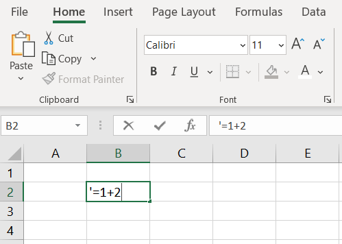
There could be a few reasons why Excel is showing the formula instead of the result. First of all, all formulas in Excel must start with the equal sign “=”. Make sure there is nothing before the equal sign. Especially if there is an apostrophe ( ‘ ) in front, in Excel (and also in other programming languages), apostrophe turns a formula or a line of code into a comment or text so the program will not run the formula or code.

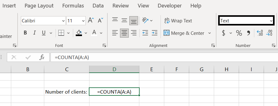
Cell is in TEXT format

This is the most common reason why Excel is showing formulas instead of the results. It happens most often when a report is exported from another system, perhaps in a CSV format. When entering a formula, it will by default be in a TEXT format:

To resolve this, change the format to General and enter the formula again:

Show Formulas is Enabled

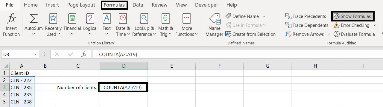
This is a less common explanation (but maybe someone is playing a prank on us, who knows?) If we go to the Formulas tab, we need to make sure Show Formulas is not selected:

Simply deselect the Show Formulas button and we shall see the end result of the formula instead of the formula itself.

The Apostrophe – All Formulas Must Start With An Equal Sign

Excel will only recognize a function or a formula and calculate it if it starts with an equal sign. That means if in a cell, we type in “1+2”, Excel will not do the calculation for us. It will simply remain as “1+2”. To have Excel do a calculation, it must start with an equal sign. Using the same example, we must enter “=1+2”.

But what if we want to enter a formula or a function into a cell and do not want Excel to calculate it? Well here we can add an apostrophe in the beginning. And the apostrophe won’t appear in the cell. What the apostrophe does is that it tells Excel this is a text and not a formula to be calculated:

Have you ever entered a value in Excel that starts with 0? For example: “007” and then Excel just removes the 0s for us and leaves the cell with 7. That is because Excel automatically recognizes “007” as a number. There are two ways we can change this and keep the 0s in front:
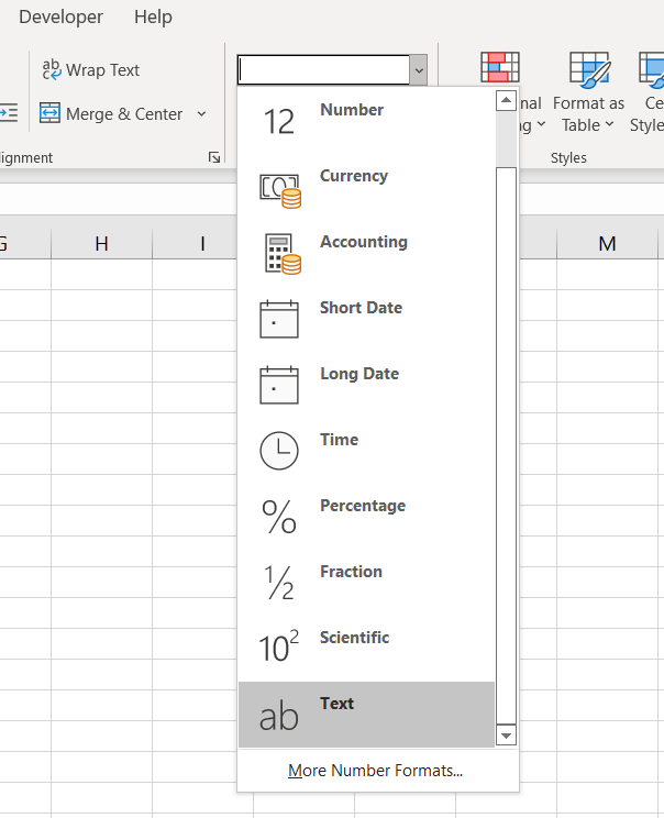
1. Change format of the cell into Text:
  
  With that, whatever we enter into the text, it will appear exactly the way we put it
2. Another way, a quicker way, would be to simply put an apostrophe before typing in the value. For example: ‘007. This will also have Excel recognize that this cell is now in a text format.
We hope this has helped you in understanding why formulas are not calculating and why Excel is showing the formulas and not calculating it. If you have gone through this article and none of these situations are applicable, feel free to leave us a comment below! We want to keep improving our content and make it more complete. So if there are other common scenarios where Excel is showing the formula instead of calculating it, please share with us!
September 11, 2021

How To Remove Empty Rows in Excel

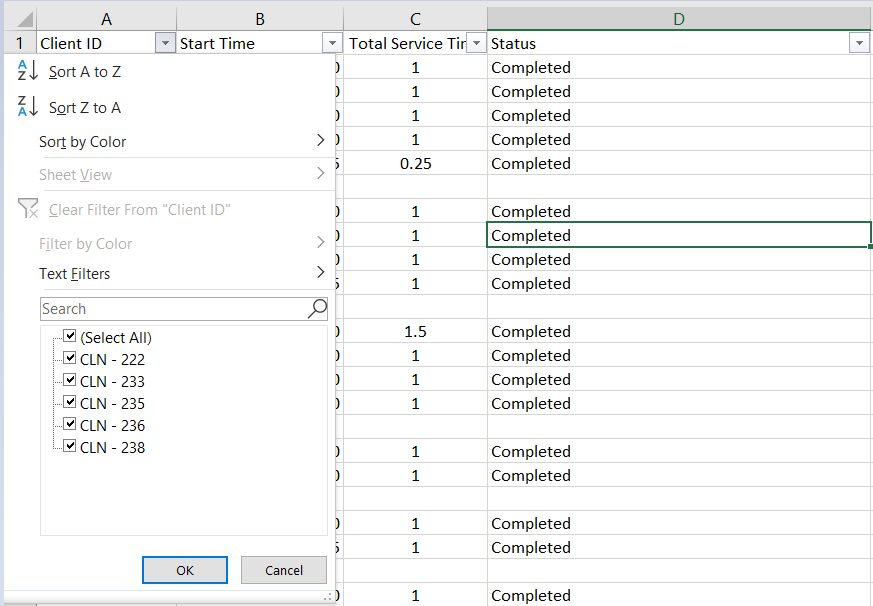
What is the best way to remove empty rows in Excel? There is a couple of different ways to do it. One way involves using Visual Basic Applications (VBA) and the other way doesn’t. In this article, we will go through both methods on how to remove empty rows.

Removing Empty Rows

The first method we will go through does not require VBA. It means this method is most likely easier to follow as no coding is required. However if removing empty rows is repetitive task that you need to do time and time again, you might want to consider creating a VBA for it. With VBA, it means the whole process can be simplified into a click of a button.

To remove empty rows:

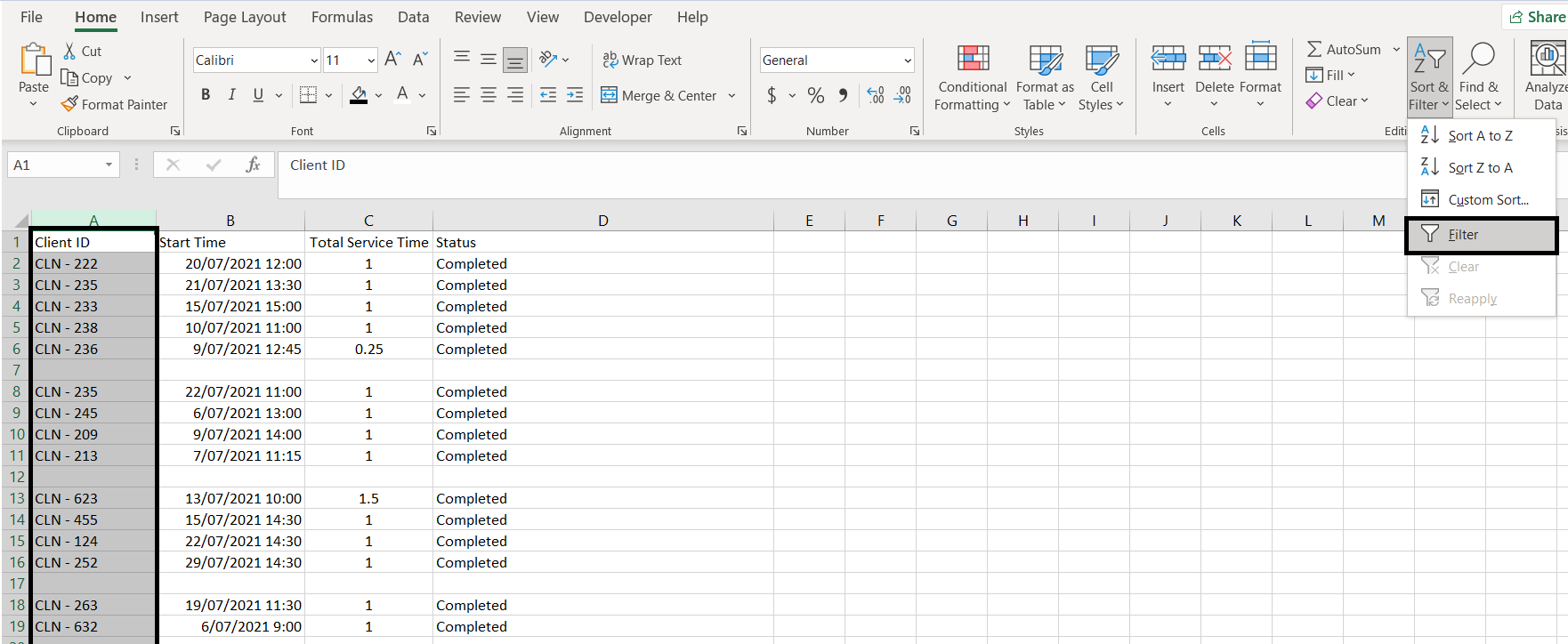
Apply filter to the whole table by first highlighting the whole column and click Filter. Alternatively use hotkey (CTRL & L) to apply Filter:

Note: it is important highlight the entire column first. Because the table is currently separated by empty rows, if we do not select the entire column, Excel will think the table ends at the first empty row. Example:
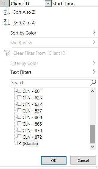
Filter to (Blanks):
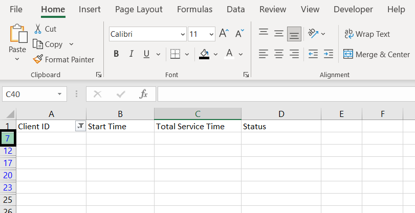
Highlight all empty rows. You can do this by first:
- Select the first empty row:
- Hold the SHIFT key
- Select the last empty row
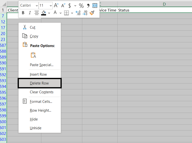
Right-click and click on Delete Row:
Remove Filter:

Here we can see that all the empty rows in the table are now removed.

Remove Empty Rows Using VBA

To use VBA, we will first need to make sure Macro/VBA is enabled. Once Macro/VBA is enabled:

Go to Developer tab and open Visual Basic
Insert a new module
Copy and paste following into the module:

Sub remove_empty_rows()
Dim i As Integer
For i = 1 To 600 ‘change 600 to the last row of the table. See below (A)
If Len (Cells(i, 1)) = 0 Then ‘Cells(row, column). In our example, the empty cell is in Column A hence it is Cells(i, 1). If it is Column B, it would be Cells(i, 2). And so on…
Rows(i).Delete
If i = 590 Then ‘change 590 to the total number of items in Column A and + 1. See below (B)
Exit For
Else
i = i – 1
End If
End If
Next i
End Sub

A) In this For loop, “For i = 1 to 600” is telling Excel to loop from number 1 to 600 and because we are putting i in Cells(i, 1), we are looping from row 1 to 600. And of course this can change depending on which row our table starts and ends.

In this example the last row of the table is 600 hence we are looping from 1 to 600

B) This number needs to be the total number of items in the column + 1. To find out, highlight the relevant column, check the “Count” at the bottom and + 1.

In this case, there are 589 items in the column hence we need 590 (589 + 1). Explanation: And this is the row number we need to tell Excel to stop and exit the For loop. This section is here to account for situations where we may have multiple consecutive blank rows. Hence every time a blank row is deleted, instead of moving onto the next row number (next i), we want to check the same row again to see if it is also blank (hence we need i = i – 1). However this can create an endless loop where “i” will never get to 600 if we keep looping i = i – 1. But if we already know that there are only 589 items in the whole column then we can confidently tell Excel to exit the For loop at row 590.

September 11, 2021

Category: Layout and Formatting

How to Freeze a Row or Column in Excel

Freeze Top Row or First Column

Freeze Row and Column

Freeze Any Row OR Column

Unfreeze Panes

Hotkeys for Freezing (or Unfreezing) Panes

How to Change and Substitute Specific Text in Excel

Find and Replace

SUBSTITUTE function

Why Is This Useful?

What You Should Use Excel For?

What is Excel Used For?

Top Reasons for Using Excel

Data Analysis and Reporting

500+ Features

VBA/Macro Coding

Import and Export Data

Benefits of Using Microsoft Excel

Effective and Easy Analysis

Collaboration

Excel iPad and Mobile Apps

Data Transformation

Bottom Line

How To Identify Duplicates in Excel

Finding Duplicates with Conditional Formatting

Finding Duplicates using COUNTIF function

Counting Unique Values

Why Is Excel Showing the Formula Instead of the Result?

Cell is in TEXT format

Show Formulas is Enabled

The Apostrophe – All Formulas Must Start With An Equal Sign

How To Remove Empty Rows in Excel

Removing Empty Rows

Remove Empty Rows Using VBA