Category: Formatting Cells

Rounding Numbers and Decimals in Excel
If you are interested in rounding numbers and decimals in Excel, you’ve found the right article. In this article, we will go through how to round decimal numbers up and down, specifying how many decimal places we want and also rounding numbers to the nearest multiples.

Rounding Decimals – ROUND, ROUNDUP and ROUNDDOWN functions

There is a few Excel built-in functions that can be used to round up/down decimals and specify how many decimal places we want. Instead of going through them separately, we will explore them together in this section so we can see the differences and know when to use each one. There are three functions:
- ROUND, ROUNDUP, ROUNDDOWN
With each function, there are two variables that needs to be entered: 1) the number that needs rounding up/down and 2) the number of decimal places to be rounded to. Here’s the difference between the three:
1. ROUND: this function runs decimals up and down in accordance with the standard mathematical rules. For numbers 1 to 4, Excel would round the decimal down. For numbers 5 to 9, Excel would round the decimal up.
2. ROUNDUP: this function is different to above because it will always round a decimal up. If we use ROUNDUP with 1.51 and round to one decimal place, it will return with 1.6.
3. ROUNDDOWN: this function is the exact opposite of ROUNDUP. It will always round a decimal down. For example if we use ROUNDDOWN with 7.99 and round to one decimal place, it will return with 7.9.
Which one you use will depend on the situation. An example of where ROUNDUP could be useful would be parking fees in a carpark. We often pay for parking by the hour and as soon as we are one minute past the hour, we will need to pay for an extra full hour. For example, if you park in a carpark for 3 hours and one minute, you don’t pay for 3 hours and one minute, you pay for 4 hours. It rounds up.

Let’s have a look at a few examples here. The first picture below, we are using ROUND, ROUNDUP and ROUNDDOWN with the decimal number on the far left and for each function, we are rounding to two decimal places:

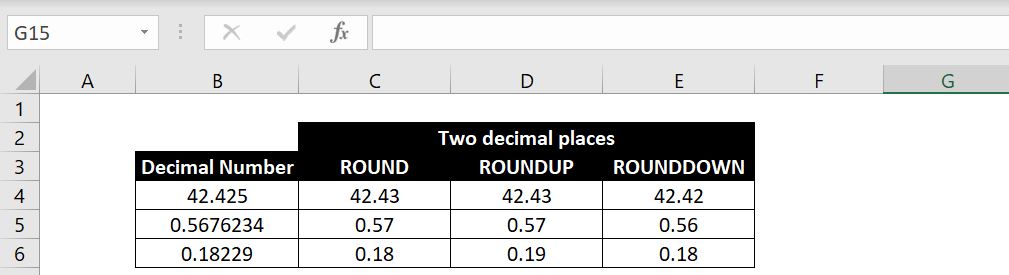
Hopefully laying the functions and results side by side, you will be able to clearly see the differences. ROUND function should operate mathematically as we would all expect. With ROUNDUP, regardless what the 3rd decimal place is, the second decimal place will always go up by one. With ROUNDDOWN, regardless what the 3rd decimal place is, the second decimal place will always remain unchanged.

Here’s another example. In this case, we want 0 decimal place:

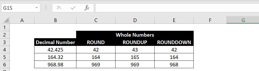
The logic is the same. With ROUNDUP, regardless what the first decimal place is, it will always round the whole number up by one. With ROUNDDOWN, regardless what the first decimal place is, the whole number will always remain unchanged.

Rounding Numbers to a Particular Multiple

In this section we will go through how to round numbers to a particular multiple. The function is MROUND. There are two variables required: 1) the number that needs rounding up/down and 2) the multiple to which the number is to be rounded to. We could specify any number and multiple and MROUND would round the number to the nearest multiple – up or down depending on which is closer.

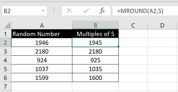
In the examples below, for each number on the left, we are rounding it to the nearest multiples of 5s. For 1946, it is closer to 1945 than it is to 1950 so Excel returned 1945:

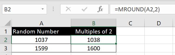
And if the number is right in the middle between the two nearest multiples, it will be rounded up. In this example we are rounding each number to an even number. And in both cases, the number is rounded up to the next even number:

Choosing to Round Up or Down to a Particular Multiple

In the section and examples above, we can’t choose whether to round the number up or down. Excel does so for us depending which multiple is closer or in the situation where the number is in the middle, it rounds up to the higher multiple. What if we want to choose to always round up (or down) to the higher (or lower) multiple?

There is no built-in Excel function for this but the formula is not too complex:
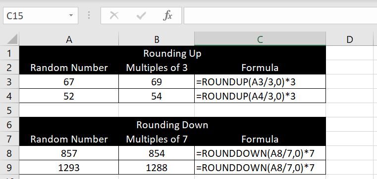
- Rounding Up:
  - = ROUNDUP(A2/n, 0) * n
  - (n: the multiple)
- Rounding Down:
  - = ROUNDDOWN(A2/n, 0) * n
  - (n: the multiple)
The logic is simple. With rounding up, whatever the number is, we first divide it by the multiple. If it is divisible then no rounding is required. If it is not divisible, there will be a decimal. And from what we went through with ROUNDUP function above, if we set decimal place to 0, the number will always be rounded up to the next whole number. For example: 22.3 will become 23, and then we can multiply 23 by the multiple. This will always round the number up to the next multiple.

Same logic with ROUNDDOWN. Whatever decimal we get, the number will remain unchanged. For example: 122.43 becomes 122, and then we multiple 122 by the multiple. This will always round the number down to the lower multiple.

See example below:
March 6, 2023
How to Separate Names in Excel
How can we separate names in Excel into first names and surnames? And what if some names have middle names in them and some don’t? In this article we will go through two different ways on how to do that in Excel. The first method we go through is to use Text to Columns and is a quicker solution. And the second method is to do this using a combination of formulas.

Separate Names Using Text to Columns

When using Text to Columns, we need to first make sure the adjacent column(s) are blank.

To separate the names using Text to Columns:
1. Highlight the list of names we would like to separate
2. Go to Data tab at the top and click on Text to Columns
3. With the Convert Text to Columns Wizard pop up, make sure “Delimited” is selected for Step 1 and click Next.
4. For Step 2, make sure Space is selected:
5. Click Finish
And Excel will return with following result:

Column A is the list first names. But the last name could be in Column B or C depending if the person has a middle name or not. To get a full list of the last names, we can add a formula in Column D:

=IF(C2>0, C2, B2)

It’s a simple formula. What it does is it checks if there’s a value in Column C. If Column C is blank, the value in Column B will be returned.

As a final touch, before removing data in Columns B and C:
1. Highlight the list of last names in Column D
2. Copy & Paste Values
This will remove the formulas and then we can delete Columns B and C. We will be left with:

Separate Names Using Formulas

Using formulas to separate first and last names is a little more complicated. However you could also just copy and paste the formulas below.

First Names

First names are a lot easier. We need to use the FIND and LEFT functions. First we find out where the first space is in the full name and we use the LEFT function to return all the characters to the left of it:

=LEFT(A2, FIND(” “, A2)-1)

The reason why we need to minus one after the FIND function is because we don’t want Excel to return the space as well. To prevent that, we FIND the location of the space and use the LEFT function to return characters up to but not including the space.

Last Name

This one is a bit trickier because some names have middle names and some don’t. To do this, we need a combination of RIGHT, FIND, LEN and SUBSTITUTE functions. To break this down, there are two scenarios here: names with middle names and names without middle names

Names Without Middle Names

For names without middle names, it works very much like first names. Except, we will be using the RIGHT function:

=RIGHT(A2, LEN(A2)-FIND(” “, A2))

First we FIND out where the space is in the full name: FIND(” “, A2). And then we find out how many characters there are in total with the full name: LEN(A2). We then minus the two to work out how many characters there are from the space to the end of the name: LEN(A2)-FIND(” “, A2). And this is the number of characters we want the RIGHT function to return.

Names With Middle Names

For names with middle names, we need to find the location of the second space (the one between the middle name and the last name). To do that, we first SUBSTITUTE the first space another character and then we can use the FIND function to look for the location of the second space:

=FIND(” “, SUBSTITUTE(A3,” “, “@”, 1)

For example, the SUBTITUTE function change “Mark James Williams” to “Mark@James Williams”. The FIND function will then be able to find the location of the space between the middle name and the last name.

After we find the location of that space, the rest is the same. We use LEN to work out the total number of characters in the full name. We then subtract the location of that space from the total number of characters. This will tell us how many characters there are with the last name:

=RIGHT(A5, LEN(A5)-FIND(” “, SUBSTITUTE(A5, ” “, “@”, 1)))

Putting Everything Together

So now we’ve worked out both scenarios, we just need to see which formula to use in each scenario. That is, to use the first formula if there is no middle name and to use the second formula if there is a middle name. And the difference between the two is the number of spaces there are in the full name. A full name with two spaces would have a middle name. And a full name with only one space would have no middle name.

We can work this out by first removing the space(s) with the SUBSTITUTE function – to swap ” ” with “”. We can then compare the number of characters before and after.

For example, with “Ronnie O’Sullivan”;

=LEN(“Ronnie O’Sullivan) will return 17

=SUBSTITUTE(“Ronnie O’Sullivan”, ” “, “”) will return “RonnieO’Sullivan”. And =LEN(“RonnieO’Sullivan”) will return 16

And the difference:

=LEN(“Ronnie O’Sullivan”)-LEN(SUBSTITUE(“Ronnie O’Sullivan”, ” “, “”) will return 1

This would tell us there is only one space in the name “Ronnie O’Sullivan”.

Now we just need to put this into an IF function. If the formula above returns a 1, we know it does not have a middle name. Otherwise, there is a middle name:

=IF(LEN(A2)-LEN(SUBSTITUTE(A2,” “,””))=1,RIGHT(A2,LEN(A2)-FIND(” “,A2)), RIGHT(A2,LEN(A2)-FIND(” “, SUBSTITUTE(A2,” “, “@”, 1))))

And with this formula above, we can draw out the last name from a full name regardless there is a middle name or not.

Now we have two different ways to separate full names in Excel. One is to use Text to Columns and the other is to use formulas. Feel free to leave a comment below if you have any questions or comments on this article!
October 23, 2022
What You Should Not Use Excel For?
Microsoft Excel significantly refined over the past few decades. However, new features prompted people to use it in ways the program was not designed for. For one, Excel is not a database. Yet, many people use it as one. While the program can serve this function for small datasets, it can exceed Excel’s limitations as soon as a small dataset grows. Let’s find out what we should not use Excel for to avoid any unnecessary complications.

Limitations of Excel

Not a CRM

We all know that implementing a new system can be very expensive. This is why many start ups and small companies choose to use Excel spreadsheets as much as they can. However when a business, using Excel as a CRM becomes complicated.

While Excel can work well with other Microsoft Office products such as PowerPoint, Access, or Word, if a part of your business depends on non-office software, transferring information between programs can be a hassle. Sure, many systems and software have options to import/export data using Excel files which means we can export data from one system and import into another software. However almost all of these software require the spreadsheet to be in a particular format and layout. This means manual intervention will be required which also means there is room for error.

When you struggle to create seamless processes with Excel and other systems, it’s time to switch to CRM software. A dedicated CRM software can help you manage your data better. You will be able to keep complete track of your customers and finances.

Cannot Handle Too Much Data

When data files are too large, Excel can run very slowly. You can lose a file if you attempt to break the data into smaller files. In addition, many users don’t consider Excel as user-friendly. Because Excel is so flexible with what you can do with it, it is not the most intuitive system to use. So, unless you know how to use all the tricks and formulas to calculate data, Excel can do little to help you.

Risk of Human Error

Misaligned rows and missed negative signs sound harmless. However, they cause considerable damage. On average, a spreadsheet contains one error for every twenty cells with data.

Whenever you make any changes in Excel manually, there is a risk of compromising accuracy and making errors. All these mistakes can have adverse effects on the bottom line. Excel may have certain error messages and alerts in place to help us with this, however there are also situations where errors may not appear. An obvious example would simply be referencing the wrong cell in a formula.

The only way you can validate data is to double-check and re-enter information. But unfortunately, that’s a labor-intensive and time-consuming exercise. Eventually, inaccurate information will ultimately lead to making decisions that are not well-informed.

Vulnerable to Fraudulent Activities

There are many cases in which fraudulent manipulations in business Excel files resulted in million-dollar losses. Lack of security and controls is the underlying reason for this vulnerability, making it easy to alter values, formulas, and dependencies without any trouble.

Difficult to Test or Troubleshoot

It’s common to have corresponding data scattered across spreadsheets at different workstations or geographical locations. However, it’s challenging to troubleshoot or test Excel worksheets.

Even if we could identify every related file, it would take a lot of time to check formulas from one cell to another. The same problems occur when we troubleshoot any questionable data.

Limitation on Visual Representations

Although the software provides many types of charts, it still has numerous limitations.

For instance,
- Diagrams are not interactive. We can use filters only to a limited extent.
- The software can’t link diagrams to one another. Instead, it handles each diagram in the file separately when setting a filter.
- There is a limited range of visualization options and diagram types.
Unsuitable for Agile Business Practices

Individuals with little IT expertise can create spreadsheets. Over time, these spreadsheet files become personalized user-developed applications. If another individual takes over these spreadsheets, he may want to start building the same spreadsheets from scratch.

It does not Offer Collaboration Opportunities

Generally, accurate pricing depends on information collected from different individuals and departments. The final document is the outcome of multiple files, ideas, and data exchanges.

When a business has multiple offices scattered throughout a city or country, exchanging high-volume data in Excel files can be challenging through email.

This exchange is vulnerable to duplication. In some cases, it can also result in incorrect data input. Team members can’t keep track of similar files going back and forth. In some cases, they can end up sending an old version.

Slow Consolidation

Although Excel is famous for its financial reporting and analysis, using the program means a slow consolidation process. You must collect data from various files, create a summary, and submit the report to the department heads through email. You may also copy to a shared network folder or use portable storage media. The process continues until the information reaches to company’s top officials.

Does not Support Decision-Making Process

When you work in a spreadsheet-based environment, you must extract data from different sources to consolidate and summarize the information. This meaningful information helps key decision-makers design the best course of action for the company.

However, everyone involved in the process must be vigilant in maintaining data integrity. In addition, the entire process takes a lot of time and does not help when company officials need to make immediate decisions. There is less time for action when the final version arrives in such a situation.

Steep Learning Curve

It’s not uncommon to find numerous books on how to use Excel because the program is not intuitive. It contains hundreds of features that beginners may not find easy to use. Users must do their homework before becoming a pro at Excel.

Data doesn’t Update in Real-time

When using Excel spreadsheets, remember that data won’t update in real-time. That means you have to make every change manually. You or your team members must update Excel spreadsheets at the end of the day or week. In some cases, it can be a monthly practice.

That means users will need some paper records whenever they are recording information in the absence of Excel spreadsheets. These records are then entered manually for updating the sheets later. Again, this duplication of effort wastes considerable time and increases the chances of entering incorrect data.

Final Thoughts

Undoubtedly, Microsoft Excel is an excellent tool for organizing and calculating data. However, the program has less value for big organizations or large-sized businesses. Therefore, choose this program only if you think the program will be able to handle your data and you won’t have trouble entering the information manually.
October 15, 2022
Copying and Pasting in Excel
Have you ever copied a cell in Excel but when you pasted it into another cell, the value was completely different? How do copying and pasting work in Excel? Did you copy the formula or the value? There are so many different “Paste” options in Excel:

In this article, we will go through a few of them. If you would like more information on any particular one of them, leave a comment below and we will add it onto this article.

Copy & Paste Formula

Have you ever copied a cell in Excel but when you pasted it into another cell, the value was completely different? This is because by default, when we copy and paste (CTRL C and CTRL V) in Excel, we are copying what is in the formula bar. And this is not necessarily the value. Of course with relative cell referencing, the referenced cell in the formula may change but the formula will not:

We now copy B2. But when we paste into B3, we will not see “Bitcoin” in B3. Instead we will see “Tellor”. This is because instead of copying “Bitcoin”, we actually copied the formula “=A1” and because of relative cell referencing, Excel is returning the value in the left adjacent cell:

This is the copying & pasting by default in Excel and hopefully explains why when you do copying and pasting in Excel, you end up seeing a different value. So let’s explore what we need to do if we want to actually copy and paste the value.

Copy & Paste Value

There could be numerous reasons why we want to copy the value inside the cell instead of copying the formula. For example, after using VLOOKUP you now have the desired returned value. And you may want to copy the value returned, not the VLOOKUP formula. Or when you use the RAND() function, the function is triggered every time we make any changes in Excel hence we get a random number generated every time. How can we use RAND() to generate a list of random numbers once and then not have it changed from then on?

First we copy (CTRL C or right-click and select Copy) the cell or the array of cells. And then we need to right-click and select Paste Values:

We can now see in the formula bar at the top, we no longer see the formula “=RAND()” but we see the actual numbers:

Another reason to copy and paste values in Excel is that after using a function, copying and pasting values will remove the formula. This means we can then make changes to (or delete) the data in the referenced cells and it will not impact the returned values we got from the formula.

Copy & Paste Format

As the name suggests, in this case we are copying and pasting the format of a cell(s). It doesn’t matter if the cell(s) contains a formula or a string. It is the format that is being copied across. So what will be copied and pasted? It is basically everything here:

It includes the font, color of the cell, cell format (General, Number, Currency, Short Date…), alignment, etc. This is the data we have before we copy and paste format:

We then copy range A1:A6 and then paste format in C1:C6 by right-clicking and selecting the second last Paste Options:

And this is the result:

Notice that the values in C1:C6 do not change. The only thing copied and pasted across is the format. This includes the bold font, the alignment, color of the cell and so on.

Format Painter

There is another way to transfer format across from one (or a range of) cell to another:
1. Select the cell(s) which has the format you would like to copy
2. Click on Format Painter icon
3. Click on where you want the cells to have the format applied to:
Notice that with Format Painter or with Paste Formats, it doesn’t affect the column width. If you would like to copy and paste the column width, you could copy and then right-click, select Paste Special:

Select Column widths and click Ok.

Copy & Paste Transpose

Simply put, Paste Transpose allows us to transfer a set of values from column to row or from row to column. This is particularly useful when we have a large set of data. We use this most often when we need to set up a table.
1. We copy the cells we would like to transpose
2. We then right-click and select the third last Paste Options:
3. And this the result:
A couple of things to keep in mind of when using Paste Transpose:
- We cannot copy and paste transpose a whole column or row
- Copying and pasting Transpose will not work with a formula that uses relative cell referencing. It will work with strings/numbers or formulas with absolute cell referencing
This is what happens with relative cell referencing. In B2:B5, we relatively reference the cell to the left. E.g. we have “=A2” in B2, “=A3” in B3 and so on. And when we paste Transpose, we have #REF error:

We’ve covered the basics in copying and pasting in Excel. We’ve explained why sometimes you get a value you don’t expect from copying and pasting. We’ve also explored some of the most popular paste options in Paste Special. If there’s anything else you would like us to go through in this article, please leave a comment below!
September 25, 2022
Useful Hotkeys in Excel
Can you use Excel without a mouse? What are some of the functions or features you use most often in Excel? If there are features in the Excel ribbons you use frequently, you will save a lot of time if you start using hotkeys in Excel. Yes it may take time to get used to it in the beginning, but once you are used to it, it almost becomes second nature. It will then be a lot quicker than using a mouse.

In this article we will go through some useful hotkeys in Excel which we use all the time. But we notice that the shortcuts we find useful may not be useful to you. So first we will look at how you can identify what the hotkeys are for all the different features in the Excel ribbons.

As always, if you feel that we have missed anything or if there’s anything else you would like to find out, please leave a comment below.

Finding Out Different Shortcuts in Excel

Chances are that the shortcuts we find useful may not be useful to you. But did you know that you can access all the buttons in the top Excel ribbons without using a mouse?

Start by simply pressing ALT key:

After pressing the ALT key, you will see some letters or numbers appear. The letters allow us to navigate across different tabs and the numbers let us to access the buttons at the very top such as Save, Undo, etc. For example we could press ALT and then A to navigate to the Data tab:

You would probably not use this for changing font to bold, italics or adding underline because you could do CTRL B, I and U. But let’s say we would like to do Paste Special, we could press ALT > H

And press V for Paste Value

With that in mind, we will go through two examples which we most commonly use.

Adding/Removing Filter

Adding and using filter is probably one of the most used features in Excel when it comes to reporting and analysis.

The hotkey is:
- CTRL & Shift & L
We also know that adding filter is in the Home tab. And from the section above, we know we can also access the Filter button with:
- ALT > H > S > F
The two sets of hotkeys are essentially the same. Of course we have to admit CTRL + Shift + L is probably more preferred. It’s similar to asking whether we would rather use ALT > H > 1 or CTRL B.

And to remove the filter, simply press the same set of hotkeys again.

Adding/Removing Border

Adding (or removing) border is something we often do when setting up a table hence this is another hotkey which we are very familiar with. This as well is in the Home tab. The hotkey for it is:
- Adding border: ALT > H > B > A
- Removing all borders: ALT > H > B > N
- For any other border: ALT > H > B > Choose the following:
Get to End of Column/Row

To get from your current cell to the last non-empty cell whether it is up, down, left or right, simply press:
- CTRL & Up/Down/Left/Right
And the other way around works as well. If you are in an empty cell and press CTRL & Up/Down/Left/Right, you would navigate to the nearest non-empty cell. And if there’s no empty cell, you would navigate to Row 1, Row 1048576, Column A or Column XFD.

Highlighting To End of Column/Row

Highlighting from one cell to the end of the end of a column/row of a table could be tedious using a mouse when you have a large set of data. It will take a lot of scrolling. To do that, simply press:
- CTRL & Shift & Up/Down/Left/Right (depending on the direction you want to go)
Autofill or Dragging Formulas

Following on from above, once we have the range of cells highlighted, let’s have a look at how we can autofill. That is, if we have a formula in one cell and we want to drag the formula down to the bottom of the table or to the right. We will use the data below as an example:

First we need to highlight the cells where we want. Because Column B is largely an empty column, the trick would be to first move to column A, press CTRL & Down. This will bring us to the bottom of the data in Column A. Press the right-arrow key to move to Column B. Here we press CTRL & Shift & Up. Here we will highlight all the cells in Column B which we want to apply the formula to:

Once we have the cells highlighted, press CTRL D.

CTRL & D is essentially a hotkey that copies the cell directly above and pastes it in current cell. Similarly CTRL & R copies the cell directly to the left and pastes in the current cell. Hence in this case, all we are doing is copying the formula down from the very top cell all the way down to the end of the highlighted cell.

Switch Between Worksheets

To navigate between worksheets within an Excel file, we could press:
- CTRL & PageUp: to move to the previous worksheet
- CTRL & PageDown: to move to the next worksheet
Other Useful Hotkeys:
- Highlight Row: Shift & Space
- Highlight Column: CTRL & Space
- Delete Row/Column: first highlight the row or column and then press CTRL & – (minus sign)
- Insert Row/Column: CTRL & + (Or essentially CTRL & Shift & =)
- Format Cell: CTRL + 1
- Insert Current Date: CTRL & ;
What Other Hotkeys Would You Like To Know About?

What other hotkeys would you like to know about? Or what other shortcuts do you feel we should include in this article? Leave us a comment below and we will add to the list?
September 18, 2022

Split Texts in Cells Using Text To Columns

The reason why we all love Excel is because we have a lot of flexibility in formatting and manipulating data the way we want. Very often we are restricted by the systems we use in terms of how we can see and present our data. And this is why we export reports into Excel files and we can format data to the way we need them to be. For example we may need to separate a list of clients’ full names into first names and last names or we need to split a list of invoice numbers. In this article, we will explore different situations, various data types and different methods to split texts in cells.

Text to Columns

Text to Columns, as the name suggests, splits text in a cell (or a range of cells) into multiple adjacent columns.

With Text to Columns, there are two options available:

Delimited: we can pick a particular character (symbol, letter or number) and every time Excel sees that character in the cell, it will split to the rest of the text into the next column. This could be useful with splitting full names into first names and last names by setting a space as the delimiter.
Fixed Width: we can split texts by setting break lines anywhere. E.g. we can choose to split texts at the fifth character in a cell. And we can create as many break lines as we want. So e.g. we can split texts at the fifth character, the seventh character and then the twentieth character. And as you can imagine, if we want to split full names into first names and last names, this would not be very useful because different names would have different numbers of characters.

Delimited

With Text to Columns – Delimited, we can choose a character – any character we want (symbol, letter or number) and every time that character appears in the cell, Excel will split the text into another column. Here’s an example below:

In our CRM, there’s a field which has checkboxes that allow more than one selection. And when we export the data into Excel, it’s formatted as below:

The data is rather messy. For entries that have multiple selections, they are all entered into one cell. This makes it very hard to do any analysis.

But we can also see that each selection is separated by a semi-colon (;). That means we can use Text to Columns – Delimited to separate each selection:

Highlight Column A
Select the Data tab at the top and click Text to Columns
Select Delimited and click Next
Select Semicolon

Note that here we could select “Other” and enter any character we want in the box next to it. The only limitation here is that although we can select multiple delimiters listed, only one character can be entered in the “Other” box.
Click Next
Click Finish

And this will be the end result:

It is now much easier to analyse the data e.g. using COUNTA or COUNTIFS.

Here’s another example. When we copy and paste a table from PDFs to Excel, the format does not always transfer across the way we want it to:

Of course we could use Power Query instead (see more here on Power Query) to export PDFs into Excel but we could also use Text to Columns with space as the delimiter. The result will not be 100% perfect (we will need to shift the headings a bit) but it will again be a lot easier to work with the data:

With some copying and pasting, it will only take a minute or two before we can format it to a proper table:

Fixed Width

Text to Columns – Fixed Width gives us the choice to create break lines wherever we want – and as many as we want. Let’s take a look at the data below as an example. It is a list of invoice numbers and let’s say in this case, we want to separate “INV” and the invoice numbers:

Text-to-Columns-Fixed-Width-Data-Excel

In this case, Text to Columns – Delimited will not be very useful because there is nothing between “INV” and the invoice number. We could potentially use “V” as the delimiter. But you can see above in Delimiter section, when we use semicolon (;) as the delimiter, the semicolon disappears after the texts are split. This means if we use “V” as the delimiter, the end result will be “IN” and invoice number – “V” will disappear.

The best way will be to use Text to Columns – Fixed Width:

The line in between “INV” and the invoice number is the break line. And it can be inserted anywhere. In fact, we can insert more than one. We can insert as many break lines as we want. For example:

And in this case, each character (“I”, “N”, “V”, “0”…) will be split into a separate cell

But back to the example above, if we insert one break line between “INV” and the invoice number and we click “Finish”, we will get the following:

In summary, there are pros and cons with using Delimited and Fixed Width. Which one you use depends on the data you currently have and how you want to split the text.

As a final tip: we can see in the example above with Fixed Width, in using Text to Columns, we don’t necessarily have to select the whole column. Many reports we extract from systems have headings and we don’t want to split the headings. We can select the range of cells we want to split and apply Text to Columns only to those cells.

If there’s anything else you would like us to add into this article, please leave a comment below! We would like to keep improving the content in our articles.

August 28, 2022

Category: Formatting Cells

Rounding Numbers and Decimals in Excel

Rounding Decimals – ROUND, ROUNDUP and ROUNDDOWN functions

Rounding Numbers to a Particular Multiple

Choosing to Round Up or Down to a Particular Multiple

How to Separate Names in Excel

Separate Names Using Text to Columns

Separate Names Using Formulas

First Names

Names Without Middle Names

Names With Middle Names

Putting Everything Together

What You Should Not Use Excel For?

Limitations of Excel

Not a CRM

Cannot Handle Too Much Data

Risk of Human Error

Vulnerable to Fraudulent Activities

Difficult to Test or Troubleshoot

Limitation on Visual Representations

Unsuitable for Agile Business Practices

It does not Offer Collaboration Opportunities

Slow Consolidation

Does not Support Decision-Making Process

Steep Learning Curve

Data doesn’t Update in Real-time

Final Thoughts

Copying and Pasting in Excel

Copy & Paste Formula

Copy & Paste Value

Copy & Paste Format

Format Painter

Copy & Paste Transpose

Useful Hotkeys in Excel

Finding Out Different Shortcuts in Excel

Adding/Removing Filter

Adding/Removing Border

Get to End of Column/Row

Highlighting To End of Column/Row

Autofill or Dragging Formulas

Switch Between Worksheets

Other Useful Hotkeys:

What Other Hotkeys Would You Like To Know About?

Split Texts in Cells Using Text To Columns

Text to Columns

Delimited

Fixed Width