Category: Dropdown List

  • How To Set Up A Searchable Dropdown List?

    How To Set Up A Searchable Dropdown List?

    In the Dropdown List in Excel article, we went through the basics of setting up a dropdown list in Excel. This time we will go through how to make a searchable dropdown list and we will also sort the list in alphabetical order so it is easier to search through the list. And then at the end we will set up an even more complex dropdown list where the list of options changes depending on another cell and is searchable.

    Creating a Searchable List

    long-list-of-entries-excel

    As an example above, let’s say there’s a very long list of entries in column A. Creating a searchable list will make it a lot easier to look through the column. To do this, we first use the SEARCH function to look for that keyword/key phrase in the list. And then we use the ISNUMBER function to see if each item in the list returns a TRUE response or a FALSE response. TRUE means it can be found. FALSE means it cannot be found. Then we use the FILTER function so that we only see the TRUE response list. And then at the end we use the SORT function to sort the end result in alphabetical order.

    To make it easier to understand, have a look at example below:
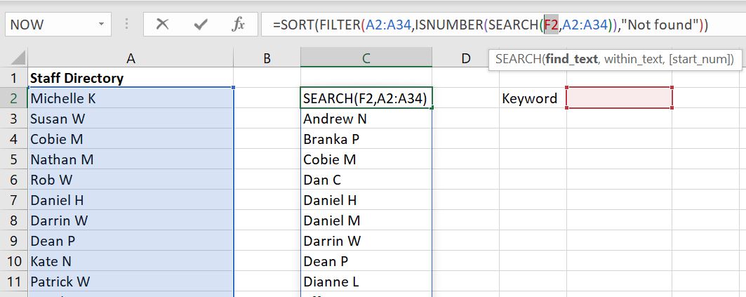
    Search-List-Full-List-Dropdown-Excel

    The formula:

    • =SORT(FILTER(A2:A34,ISNUMBER(SEARCH(F2,A2:A34)),”Not found”))

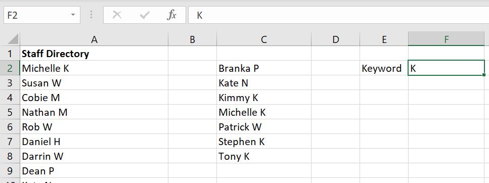
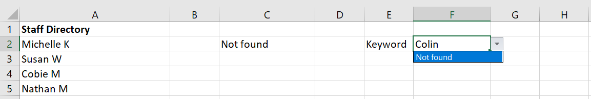
    The formula looks for what is entered in F2 (Keyword) in the A2:A34 list. If anything can be found, the A2:A34 list will be filtered to return the new list. Tip: if there is no keyword or key phrase entered at all, the full list will appear. And if nothing can be found, the list will return with “Not found”.

    Search-List-Dropdown-Excel

    Search-List-Dropdown-Not-Found-Excel

    Put this New Searchable List into a Dropdown List

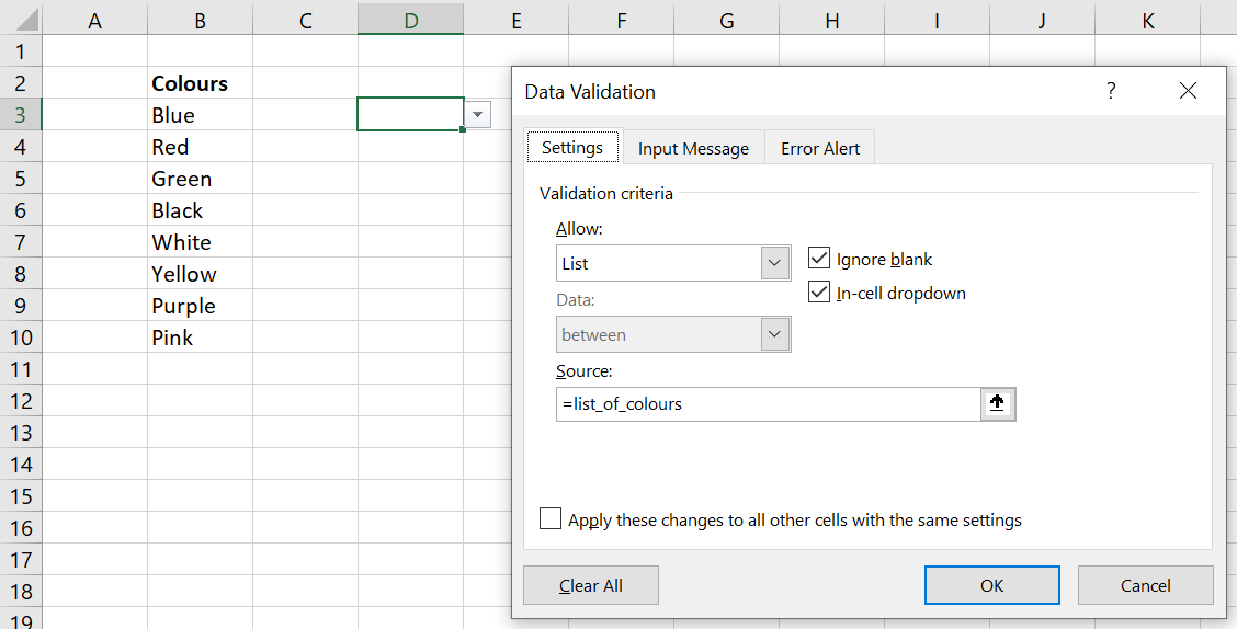
    To make this searchable list a dropdown list, it is simple. Select the cell where you want to create the dropdown list, go to Data at the top and select Data Validation:

    Dropdown-list-data-validation

    Tip: Because we don’t know how many items will be returned based on the keyword or key phrase, the list is dynamic. We know the list starts with C2 and then we can add # after it. This way Excel will include everything from C2 to the last item in the list, whatever that is.

    In the Error Alert tab, make sure the “Show error alert after invalid data is entered” is not ticked.

    Dropdown-list-error-alert-data-validation

    Now we have a dropdown list which is searchable.

    Searched-Dropdown-List-Excel

    Searched-Dropdown-List-Not-Found-Excel

    Creating a Dynamic Searchable Dropdown List

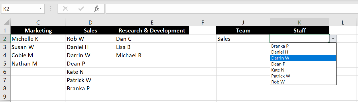
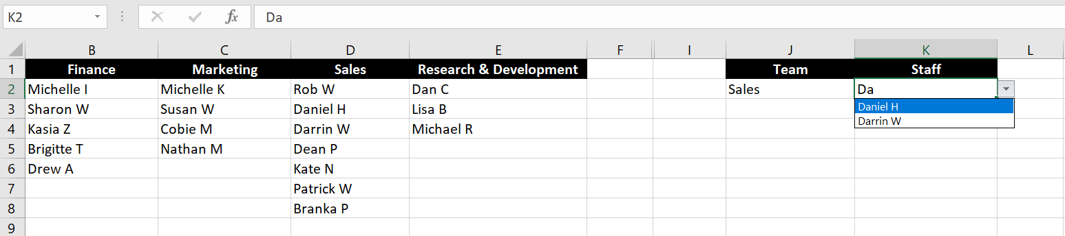
    Combining everything we’ve learned, we will now make a dropdown list where the list of entries changes depending on value of another cell and is searchable. Continuing on with the example above, in the real world a staff directory is usually separated by teams. So how can we have a dropdown list where the list of staff is different depending on which team is selected? And of course we want the list to be searchable.

    For example: the first dropdown list allows you to select one of the teams that is available across Row 1 (A1:E1):

    First-Dropdown-List-Excel

    And the second list “Staff” changes depending on which team you’ve selected in J2:

    Second-Dropdown-List-Excel

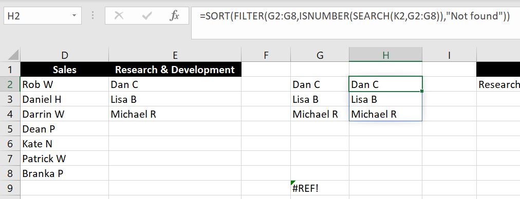
    To do this, we really only need to add one more step to above. Because there are now multiple lists available, we now need to create this one list which updates itself depending on which team is selected:

    Search-List-Depending-On-First-Dropdown-Excel

    The formula is:

    • =INDEX($A$2:$E$8,ROW($A$1:$E$8),MATCH($J$2,$A$1:$E$1,0))

    This…looks ugly. The #REF does not matter because when making this list searchable, the #REF will return a FALSE result hence it won’t show up in the final dropdown list. But the 0 will if no keyword/key phrase is added – because the full list appears when nothing is entered. To fix this, we just need to add an IF formula. IF a 0 is returned, give us blank “” instead.

    • =IF(INDEX($A$2:$E$8,ROW($A$1:$E$8),MATCH($J$2,$A$1:$E$1,0))=0,””,INDEX($A$2:$E$8,ROW($A$1:$E$8),MATCH($J$2,$A$1:$E$1,0)))

    Updated-List-Depending-On-First-Dropdown-List-Excel-index-match-no-zeroes

    As mentioned, it doesn’t matter if the #REF is there. But if you like to see a cleaner list, you can use the IFERROR formula so that any error will also return “” – blank.

    The next step is to make this new list searchable. Here we follow the exact same steps as what we’ve shown in the beginning of this article. First we search for what is entered in K2 in the new G2:G8 list. Then we see if a TRUE or FALSE response is returned. And then we filter to have a list with the TRUE responses. At the end we sort the list alphabetically.

    Search-Dynamic-List-Dropdown-Excel

    Again, we need to go into the Error Alert tab and make sure the “Show error alert after invalid data is entered” box is not selected.

    Search-New-Dynamic-List-Dropdown-Data-Validation-Excel-2

    To make the file look cleaner, you can hide column G and H. Sometimes we set this up in a separate worksheet tab and protect the sheet so no one would accidentally change or delete the formulas. For information on how to protect a worksheet, you can check out How to Password Protect an Excel File.

    Excel-Searchable-Dynamic-Dropdown-List

    We hope we have made it clear on how to make a searchable dropdown list and how to have the list changed depending on the value of another cell. If anything is not clear, feel free to leave a comment below!

  • Dropdown Lists in Excel

    Dropdown Lists in Excel

    How can we add a dropdown list in Excel? What if we want the dropdown list to change depending on another cell value? In this article, we will go through how to add a dropdown list in Excel. We will also look at how to have a dropdown list that users can overwrite. In addition we will go through how to add an alert or warning message when users wish to enter free text into a cell with dropdown list. And before the end, we will go through how to remove a dropdown list and also discuss the benefits of using a dropdown list.

    How To Add A Dropdown List

    We will first go through how to add a basic dropdown list:

    1. Select the cell or cells we would like to create a dropdown list for
    2. Go to Data tab at the top
    3. Click on Data Validation (see image below):

      data-validation-dropdown-list
    4. Allow: List
    5. For Source, there is a few ways we can decide what should be in the dropdown list:
      1. Type out the list and separate each option with a comma (e.g. blue, red, yellow, green)
      2. Select the cells as a reference if the list is in the file. A benefit of this is that if the values of those cells are updated, the dropdown list will update automatically (see image below):

        data-validation-dropdown-list-source
      3. Reference by using Name Managers is also an option. Remember to put an equal sign before the name manager otherwise the name manager itself will become the dropdown list:

        data-validation-dropdown-list-name-manager

    We definitely prefer using Name Managers or cell references. Whichever way you would like to create your dropdown list, here’s the result:

    A Dropdown List That Can Be Overwritten

    With a dropdown list, you may or may not want the free text option to type in whatever you want into the cell. This means you can have either:

    1. A dropdown list and users must only select from the list
    2. A dropdown list but also give users the option to enter free text

    There are definitely benefits with not allowing users to enter free text but there are times when it might be helpful. For example, it could be useful to have the most common selections available in the dropdown list but also allow users to type in their responses, should the value they want to enter is not in the dropdown list. By default, an error message will appear if we try to enter a value that is not listed as one of the options in the dropdown list:

    Dropdown-List-Error-Excel

    Luckily, we can change this. First, we go back into Data Validation. And in the Error Alert tab, make sure the “Show error alert after invalid data is entered” is not selected:

    Excel-Error-Alert-Excel

    Click OK to save.

    Once that is done, we can now enter anything we want into the cell:

    Dropdown-Free-Text-Excel

    Alert or Warning Message

    In the section above, we went through how we can allow free text from users when there is a dropdown list. In this section we will show how we can allow users to enter free text into a cell that has a dropdown list but have a warning or alert message pop up whenever free text is entered.

    To do this, we go back into Data Validation > Error Alert tab:

    Warning-Message-Dropdown-List-Excel

    This time we leave the “Show error alert after invalid data is entered” box ticked and underneath that, we have:

    • Style: Warning
    • Error message: this is a free text field. You can have whatever error message pop up whenever invalid data is entered

    Now let’s test this out again. When we enter “Brown” which is not one of the options in the dropdown list, we will see the following message:

    Alert-Message-Excel-Dropdown-List

    The benefit of this is that it would encourage users to check what they’ve put in. But it is not so restrictive that entering a different value becomes impossible.

    How to Remove a Dropdown List

    Removing a dropdown list is very simple. Simply go back into Data Validation and for Allow:

    • Instead of List, select Any value:

    Remove-Dropdown-List-Excel

    This will remove the dropdown list and we will be allowed to enter any value we want into the cell.

    The biggest benefit with using dropdown list is it limits what users can enter into the cell. It gives more predictable results and makes data easier to collate and analyze later on. Imagine you have a spreadsheet which will be used by several different users, even for simple data where you expect people to give a rating out of 10, you could end up getting data such as “1” or “one”, “unsure”, “low”, “19”. Data like that will take a long term to clean up.

    This is it so far with dropdown list. We hope you find this article useful. If we have missed anything or if you have any further questions on creating a dropdown list, please leave a comment below!